15.0 Taguchi Loss Function Analysis - VAS Documentation Manual

The Taguchi loss function is a well-known analytic methodology that quantifies the economic loss associated with the deviation of a performance measurement Y from a pre-specified, optimal target value T. The loss is directly related to the common and assignable causes creating the variation in Y. The methodology has been adopted and modified to form the foundation for the analysis of the contribution of the cause system components $\{\mu,\ \rho_{k},\ \alpha_{i},\ \beta_{j},\ {\alpha\beta}_{ij},\tau_{t},\ {\rho\tau}_{kt},and\ \varepsilon_{ktn}'\}$ to the variation affecting the performance measurement Y.

15.1 The Basic Theory for the Taguchi Loss Function – L(Y)¶

We first present the basic theory for the Taguchi loss function for the case where the performance measurement Y is produced by a single, constant cause system of variation associated with a statistical density function $f.$ Note that if the process is associated with a cause system that is producing uncontrolled variation in the performance measurement, then the loss is unpredictable. This is another important reason why bringing a process into a state of statistical control is so important.

Let µ denote the mean value for Y, and let σ denote the standard deviation for Y. If $\left\{ Y_{1},\ Y_{2},\ldots,\ Y_{n},\ldots,Y_{N} \right\}$ denotes a random sample of size N from the process, then the performance measurement Y for a constant cause system can be modeled as in Equation 15-1.

(equation picture — LaTeX to be added)

Equation 15-1. The Basic Statistical Model for the Taguchi Loss Function Analysis

Let T denote the target value for Y where T is defined to be the “optimal” value for Y from a customer or production perspective. For processes where the concept of an optimal target value is not applicable, the target T is set to the overall average value ${\overline{Y}}_{..}$ for the performance measurement Y.

Although it may not be known exactly, it is reasonable to assume that some economic loss is incurred as Y deviates from T. That is, the loss is a function of the difference Y-T, and by definition the loss is minimized when Y = T. For example, consider filling medication orders in a pharmacy, and let Y be the daily error rate measured as the percent of orders filled incorrectly. Clearly the optimal target value is T = 0%. The larger the error rate (i.e., the further the error rate Y deviates from 0), the larger the loss to the organization because the errors must be discovered and corrected which is costly. In addition, if the errors are not discovered and corrected, the risk of patient injury and liability increases. As another example, consider a process designed to fill cups with a liquid product. If the “Label Claim” is 237 grams, then the further the value of the product fill weight Y deviates from 237 grams, the larger the loss to the organization. This loss is due to either wasted product associated with overfilled cups or the risk of customer dissatisfaction associated with under filled cups.

The loss associated with Y is denoted by L(Y). Figure 15-1 is a graphical representation of the form of a typical two-sided loss function. Note, that without loss of generality, we can assume that the loss is zero at Y = T since by definition the loss is minimized at T. This is true because if $L(T) \neq 0$ , we can redefine the loss function to be

L^{*}(Y) = L(Y) - L(T)

in which case L*(T) = 0. The loss function can also be single-sided (i.e. the value of the loss function can be 0 to the left of the target value, or it can be 0 to the right of the target value) as illustrated in Figure 15-2. The loss function can also be asymmetric.

Figure 15-1. The Generic Form for the Loss Function L(Y)

Figure 15-2. The One-Sided Loss Function

What is interesting, and of great practical importance, is that the actual form of the loss function L does not need to be known. Only two mild assumptions are made about the nature of the loss function L(Y).

The loss is minimized when Y = T, and therefore without loss of generality we can assume L(T) = 0.
L(Y) increases monotonically as Y deviates from T.

Applying the mathematical theory of Taylor series approximations, it is known that any reasonably smooth function L can be approximated by the following equation.

L(Y) \approx L(T) + \ L'(T)(Y - T) + \ \frac{L"(T)}{2}{(Y - T)}^{2} \tag{15-2}

Equation 15-2. The Taguchi Loss Function

where $L'(T)and\ L^{''}(T)$ are the first and second derivatives of L evaluated at Y=T. Applying the fact that L is minimized at Y=T, it follows that both L(T) = 0 and $L'(T) = 0.$ Therefore,

L(Y) \approx \frac{L"(T)}{2}(Y - T)^{2} = C(Y - T)^{2} \tag{15-3}

Equation 15-3. The Approximate Taguchi Loss Function

where

C = \frac{L"(T)}{2}\ .

This analysis demonstrates that the loss is proportional to the squared deviation $(Y - T)^{2}$ .

Under the assumption that the performance measurement Y is produced by the density function $f$ , Figure 15-3 illustrates the relationship between the loss function L(y) and the density function f(y).

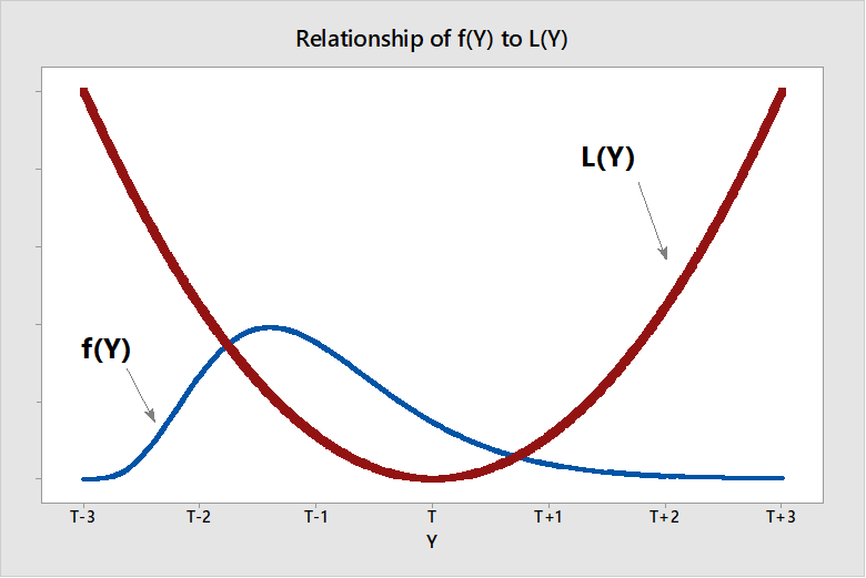
Figure 15-3. The Relationship Between the Loss Function and Density Function — **Figure 15-3.** The Relationship Between the Loss Function and Density Function

The process mean, denoted by µ, is defined by Equation 15-4.

\mu = \int_{- \infty}^{+ \infty}{yf(y)dy} \tag{15-4}

Equation 15-4. The Mean for the Distribution of Y

The process variance, denoted by σ², is defined by Equation 15-5.

\sigma^{2} = \int_{- \infty}^{+ \infty}{{(y - \mu)}^{2}f(y)dy\ \ } \tag{15-5}

Equation 15-5. The Variance for the Distribution of Y

The average or expected loss, denoted by EL, is defined by Equation 15-6.

EL = \ \int_{- \infty}^{+ \infty}{L(y)f(y)dy \propto \ \int_{- \infty}^{+ \infty}{C(y - T)}^{2}f(y)\ dy\ \ \ \ \ \ \ \ \ \ \ \ \ \ \ \ \ \ \ \ \ \ \ \ \ \ \ \ } \tag{15-6}

Equation 15-6. The Expected Loss for Y

But,

\int_{- \infty}^{+ \infty}{C(y - T)}^{2}f(y)dy

= \ \ \int_{- \infty}^{+ \infty}{C(y - \mu + \ \mu - T)}^{2}f(y)dy

= \ \ C\int_{- \infty}^{+ \infty}{\lbrack(y - \mu)^{2} + 2(y - \mu)(\mu - T) + (\mu - T)^{2}}\rbrack\ f(y)dy

= C\left\lbrack \int_{- \infty}^{+ \infty}(y - \mu)^{2}f(y)dy\ + 2(\mu - T)\int_{- \infty}^{+ \infty}{(y - \mu)f(y)dy\ +}\ \int_{- \infty}^{+ \infty}(\mu - T)^{2}f(y)dy\ \right\rbrack

= C\left\lbrack \int_{- \infty}^{+ \infty}(y - \mu)^{2}f(y)dy\ + \ (\mu - T)^{2}\int_{- \infty}^{+ \infty}{f(y)dy}\ \right\rbrack

= \ C\left\lbrack \sigma^{2} + (\mu - T)^{2} \right\rbrack

since $\int_{- \infty}^{+ \infty}{(y - \mu)f(y)dy = 0}$ and $\int_{- \infty}^{+ \infty}{f(y)dy = 1}$ .

The important summary conclusion resulting from this fairly complex mathematical analysis is the following.

“For any constant cause system associated with the statistical density f that admits a mean µ and standard deviation σ, the average loss incurred is directly proportional to the process variance $\sigma^{2}$ plus the square of the deviation of the process mean µ from the target value T.”

This conclusion is summarized in Equation 15-7.

EL \propto \left\lbrack \sigma^{2} + (\mu - T)^{2} \right\rbrack \tag{15-7}

Equation 15-7. The Components of the Taguchi Loss Function

These theoretical results have great practical value. Note that for a single stable process of interest, the value for the unknown proportionality constant C is not important. No matter the value of C, the average loss is minimized by minimizing σ² and (µ - T)². Therefore, we can assume for convenience that $C = 1$ .

The loss function analysis clearly demonstrates that in order to minimize the average loss, focus must be placed on:

bringing the process variation into a state of statistical control so that the loss is predictable;
bringing the process mean on target (i.e., moving µ as close as possible to T); and
minimizing the process variance σ².

15.2 Extending the Loss Function Methodology to Analytic Studies¶

Consider a process in which the data have been placed into R = KxT rational subgroups based on the combinations of the process design conditions and production time as in Figure 15-4. Each rational subgroup is associated with its own cause system of variation defined by its density function $f_{kt}$ , mean $\mu_{kt}$ and standard deviation $\sigma_{kt}$ . Therefore, the kt^th rational subgroup has its own expected loss function given by Equation 15-8.

{EL}_{kt} = \left\lbrack \sigma_{kt}^{2} + \ \left( \mu_{kt} - T \right)^{2} \right\rbrack \tag{15-8}

Equation 15-8. The Taguchi Loss Function for the ktth Rational Subgroup

If the kt^th rational subgroup produces a proportion $p_{kt}$ of the process output, then the expected loss EL for the process is the average of the rational subgroup expected losses given in Equation 15-9.

EL = \sum_{k = 1}^{K}{\sum_{t = 1}^{T}{p_{kt}\left\lbrack \sigma_{kt}^{2} + \left( \mu_{kt} - T \right)^{2} \right\rbrack}\ } \tag{15-9}

Equation 15-9. The Weighted Taguchi Loss Function

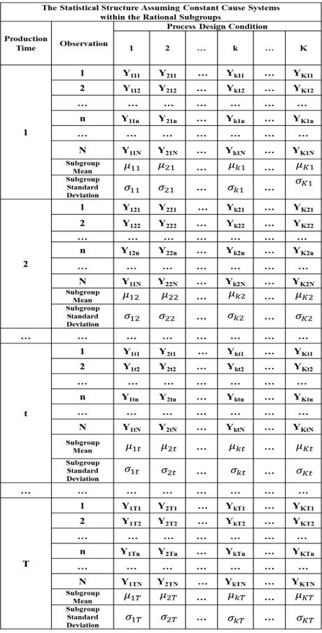
Figure 15-4. The Statistical Structure for a Constant Cause System of Variation — **Figure 15-4.** The Statistical Structure for a Constant Cause System of Variation

In most applications each rational subgroup produces the same proportion of the process output so $p_{kt}$ = 1/KT, and the expected loss is given by Equation 15-10.

EL = \frac{1}{KT}\sum_{k = 1}^{K}{\sum_{t = 1}^{T}\left\lbrack \sigma_{kt}^{2} + \left( \mu_{kt} - T \right)^{2} \right\rbrack\ } \tag{15-10}

Equation 15-10. The Unweighted Taguchi Loss Function

15.2.1 The Taguchi Loss Function for the Re-Parameterized VAS Model¶

We can also express the loss function using the re-parameterized model in Equation 15-11.

{Y_{ktn} = \ \mu + \rho_{k} + \tau_{t} + {\rho\tau}_{kt} + \varepsilon_{ktn}\ \ k = 1,\ 2,\ \ldots,K\ \ t = 1,2,\ \ldots,T\ \ \ }{\ \ \ \ \ \ \ \ \ \ \ \ \ \ \ \ \ \ \ \ \ \ \ \ \ \ \ \ \ \ \ \ \ \ \ \ \ \ \ \ \ \ \ \ \ \ \ \ \ \ \ \ \ \ \ \ \ \ \ \ \ \ \ \ \ \ \ \ n = 1,2,\ldots,\ N_{kt}\ } \tag{15-11}

Equation 15-11. The Re-Parameterized VAS Model

In this case the expected loss associated with the kt^th rational subgroup is given by Equation 15-12.

{EL}_{kt} = \ \sigma_{kt}^{2} + \left( \mu + \rho_{k} + \tau_{t} + {\rho\tau}_{kt} - T \right)^{2} \tag{15-12}

Equation 15-12. Expected Loss Function for the ktth RSG for the Re-Parameterized Model

Expanding the terms in Equation 15-12, we obtain the following form for ${EL}_{kt}$ .

{EL}_{kt} = \ \sigma_{kt}^{2} + {(\mu - T)}^{2} + 2(\mu - T)\rho_{k} + 2(\mu - T)\tau_{t} + 2(\mu - T){\rho\tau}_{kt} + \rho_{k}^{2} + 2\rho_{k}\tau_{t} + 2\rho_{k}{\rho\tau}_{kt} + \tau_{t}^{2} + 2\tau_{t}{\rho\tau}_{kt} + {\rho\tau}_{kt}^{2}

The expected loss for the process is then given by

EL = \ \ \frac{1}{KT}\sum_{k = 1}^{K}{\sum_{t = 1}^{T}\left\lbrack \sigma_{kt}^{2} + (\mu - T)^{2} + 2(\mu - T)\rho_{k} + 2(\mu - T)\tau_{t} + 2(\mu - T){\rho\tau}_{kt} + \rho_{k}^{2} + 2\rho_{k}\tau_{t} + 2\rho_{k}{\rho\tau}_{kt} + \tau_{t}^{2} + 2\tau_{t}{\rho\tau}_{kt} + {\rho\tau}_{kt}^{2}\ \ \right\rbrack}

Therefore, given the constraints

\sum_{k = 1}^{K}\rho_{k} = 0,\ \sum_{t = 1}^{T}\tau_{t} = 0,\ \sum_{k = 1}^{K}{\rho\tau}_{kt} = 0,\ \sum_{t = 1}^{T}{\rho\tau}_{kt} = 0

the expected loss is given in Equation 15-13.

EL = \ (\mu - T)^{2} + \frac{1}{KT}\sum_{k = 1}^{K}{\sum_{t = 1}^{T}\sigma_{kt}^{2}} + \frac{1}{K}\sum_{k = 1}^{I}\rho_{k}^{2} + \ \frac{1}{T}\sum_{t = 1}^{T}\tau_{t}^{2} + \ \frac{1}{KT}\sum_{k = 1}^{K}{\sum_{t = 1}^{T}{\rho\tau}_{kt}^{2}} \tag{15-13}

Equation 15-13. The Taguchi Loss Function for the Re-Parameterized Model

15.3 Components Contributing to the Total Variation in Y¶

It can be seen from Equation 15-13 that there are five components that contribute to the loss. The following meanings can be assigned to these five components.

${(\mu - T)}^{2}$ measures the contribution to loss due to the global centering of the overall process at the value µ.
The term $\frac{1}{KT}\sum_{k = 1}^{K}{\sum_{t = 1}^{T}\sigma_{kt}^{2}}$ measures the contribution to loss due to the unexplained variation occurring within the rational subgroups.
The term $\frac{1}{K}\sum_{k = 1}^{K}\rho_{k}^{2}$ measures the contribution due to the assignable causes associated with the process design conditions operating globally over all the production times.
The term $\frac{1}{T}\sum_{t = 1}^{T}\tau_{t}^{2}$ measures the contribution due to the assignable causes associated with production time operating globally over all of the process design conditions.
The term $\frac{1}{KT}\sum_{k = 1}^{K}{\sum_{t = 1}^{T}{\rho\tau}_{kt}^{2}}$ measures the contribution due to the interaction effects between the process design conditions and production time.

15.4 Estimating the Component Contributions to the Taguchi Loss Function¶

The expected loss function depends upon the rational subgroup means $\left\{ \mu_{kt} \right\}$ and subgroup standard deviations $\left\{ \sigma_{kt} \right\}$ . In order to estimate the expect loss, we need to estimate these parameters, and the method of estimation depends upon the sampling design state associated with the rational subgrouping structure in Figure 15-4.

15.4.1 Estimating the Expect Loss for Sampling Design States 1 and 4¶

The subgroup means are simply estimated using the rational subgroup sample averages.

$> {\widehat{\mu}}_{kt} = \frac{1}{N_{kt}}\sum_{n = 1}^{N_{kt}}Y_{ktn} = \ {\overline{Y}}_{kt.} >$

The following components of the loss function are then estimated as follows.

$\widehat{\mu} = \frac{1}{KT}\sum_{k = 1}^{K}{\sum_{t = 1}^{T}{\widehat{\mu}}_{kt}} = \ \frac{1}{KT}\sum_{k = 1}^{K}{\sum_{t = 1}^{T}{\overline{Y}}_{kt.}} = {\overline{\overline{Y}}}_{..}$
${\widehat{\rho}}_{k} = {\overline{Y}}_{k.} - \ {\overline{\overline{Y}}}_{..}$
${\widehat{\tau}}_{t} = {\overline{Y}}_{.t} - \ {\overline{\overline{Y}}}_{..}$
${\widehat{\rho\tau}}_{kt} = {\overline{Y}}_{kt} - {\overline{Y}}_{k.} - {\overline{Y}}_{.t} + \ \ {\overline{\overline{Y}}}_{..}$

The rational subgroup variance $\sigma_{kt}^{2}$ is estimated by the rational subgroup sample variance defined in Equation 15-14.

{\widehat{\sigma}}_{kt}^{2} = S_{kt}^{2} \tag{15-14}

Equation 15-14. Estimate of the RSG Variances for ADS 1

where $S_{kt}$ is the rational subgroup standard deviation defined in Equation 15-15.

S_{kt} = \sqrt{\frac{\sum_{n = 1}^{N_{kt}}\left( Y_{ktn} - {\overline{Y}}_{kt.} \right)^{2}}{N_{kt} - 1}} \tag{15-15}

Equation 15-15. RSG Sample Standard Deviation

The expected loss is then estimated as in Equation 15-16.

\widehat{EL} = \left( {\overline{Y}}_{..} - T \right)^{2} + \frac{1}{KT}\sum_{k = 1}^{K}{\sum_{t = 1}^{T}S_{kt}^{2}} + \frac{1}{K}\sum_{k = 1}^{K}{\left( {\overline{Y}}_{k.} - {\overline{\overline{Y}}}_{..} \right)^{2} + \frac{1}{T}}\sum_{t = 1}^{T}\left( {\overline{Y}}_{.t} - {\overline{\overline{Y}}}_{..} \right)^{2} + \frac{1}{KT}\sum_{k = 1}^{K}{\sum_{t = 1}^{T}\left( {\overline{Y}}_{kt.} - {\overline{Y}}_{k.} - {\overline{Y}}_{.t} + {\overline{\overline{Y}}}_{..} \right)^{2}} \tag{15-16}

Equation 15-16. The Estimated Expected Loss for SDS 1 and SDS 4

15.4.2 Estimating the Expect Loss for Sampling Design States 2, 3, 5 and 6¶

As discussed in previous sections, for sampling design states 2, 3, 5, and 6 there is only a single observation in some , or all, of the rational subgroups. Therefore, in these states, there is no direct way to estimate some, or all, of the rational subgroup standard deviations $\left\{ \sigma_{kt} \right\}$ . This creates difficulty with respect to separating and measuring the contributions of the PCDxPT interaction and the unexplained variation to the total loss.

In this case the contribution of the unexplained causes of variation to the expected loss is defined to be the sample variance for the R2 residuals given in Equation 15-17.

{\widehat{\sigma}}^{2} = \ S_{R2}^{2} \tag{15-17}

Equation 15-17. Contribution of Unexplained Causes for ADS 2, 3, 5 and 6

The contribution due to the PDCxPT interaction effects is based on the following logic. The total expected loss for the process is estimated using Equation 15-18 where S is the overall standard deviation for the performance measurements or equivalently the R1 residuals.

Total\ Eloss = \ \left( {\overline{Y}}_{..} - T \right)^{2} + S^{2} \tag{15-18}

Equation 15-18. The Total Process Loss

If the contributions to the total loss due to the process mean, PDC main effects, PT main effects process and the unexplained causes of variation are subtracted from the total loss, the remainder must be due, at least approximately, to the PDCxPT interaction effects. So the contribution due to the PDCxPT interaction effects is given by Equation 15-19

EL(PDCxPT) = \ {\lbrack\left( {\overline{Y}}_{..} - T \right)}^{2} + S^{2}\rbrack - \left( {\overline{Y}}_{..} - T \right)^{2} - \frac{1}{K}\sum_{k = 1}^{K}{\left( {\overline{Y}}_{k.} - {\overline{\overline{Y}}}_{..} \right)^{2} - \frac{1}{T}}\sum_{t = 1}^{T}\left( {\overline{Y}}_{.t} - {\overline{\overline{Y}}}_{..} \right)^{2} - S_{R2}^{2} \tag{15-19}

Equation 15-19. The PDCxPT Contribution to Loss

Since the $\left( {\overline{Y}}_{..} - T \right)^{2}$ term cancels out, the contribution of the PDCxPT interaction terms to the loss reduces to Equation 15-20.

EL(PDCxPT) = \ S^{2} - \frac{1}{K}\sum_{k = 1}^{K}{\left( {\overline{Y}}_{k.} - {\overline{\overline{Y}}}_{..} \right)^{2} - \frac{1}{T}}\sum_{t = 1}^{T}\left( {\overline{Y}}_{.t} - {\overline{\overline{Y}}}_{..} \right)^{2} - S_{R2}^{2} \tag{15-20}

Equation 15-20. Contribution of the PDCxPT Interaction to Loss for SDS 2, 3, 5 and 6

If $EL(PDCxPT)\ < 0,$ then $EL(PDCxPT)$ is set to 0. The final form for the estimated expected loss for SDS 2, 3, 5 and 6 is given in Equation 15-21.

\widehat{EL} = \left( {\overline{Y}}_{..} - T \right)^{2} + S_{R2}^{2} + \frac{1}{K}\sum_{k = 1}^{K}{\left( {\overline{Y}}_{k.} - {\overline{\overline{Y}}}_{..} \right)^{2} + \frac{1}{T}}\sum_{t = 1}^{T}\left( {\overline{Y}}_{.t} - {\overline{\overline{Y}}}_{..} \right)^{2} + EL(PDCxPT) \tag{15-21}

Equation 15-21. Estimated Expected Loss for SDS 2, 3, 5 and 6

15.5 The Contribution of the Process Design Factors to the Expected Loss¶

The total contribution due to the process design conditions (PDC) is given in Equation 15-22.

\frac{1}{K}\sum_{k = 1}^{K}\left( {\overline{Y}}_{k.} - {\overline{\overline{Y}}}_{..} \right)^{2} \tag{15-22}

Equation 15-22. The Contribution of the Process Design Conditions to the Expected Loss

When there are multiple process design factors creating the process design conditions, the PDC contribution to the expected loss can be decomposed into the contributions due to the individual process design factor main effects and the total contribution due to all of the interaction effects among the process design factors in the following way.

Consider the case where there are M process design factors $\left\{ F_{1},F_{2},\ldots,F_{m},\ldots,F_{M} \right\}$ , and factor $F_{m}$ occurs at I levels. The factor main effects are presented in Equation 15-23.

Main\ Effect\ for\ Level\ i\ of\ PD\ Factor\ F_{m} = \ {\overline{R5}}_{\ldots i\ldots}\ \ i = 1,\ 2,\ldots,I \tag{15-23}

Equation 15-23. Main Effects for Process Design Factor

The loss due to the main effects for process design factor $F_{m}$ is given in Equation 15-24.

Loss\left( F_{m} \right) = \frac{1}{I}\sum_{i = 1}^{I}\left( {\overline{R5}}_{\ldots i\ldots} \right)^{2} \tag{15-24}

Equation 15-24. The Loss Due to the Main Effects of Process Design Factor Fm

The total loss due to the process design factor main effects is given in Equation 15-25.

Total\ Loss\ Associated\ with\ PD\ Main\ Effects = \ \sum_{m = 1}^{M}{{Loss(F}_{m})} \tag{15-25}

Equation 15-25. Total Loss Due to Process Design Factor Main Effects

The difference in the loss due to the process design conditions (PDC) presented in Equation 15-22 and the total loss due to the process design factor main effects in Equation 15-25 is the loss due to all of the process design factor interaction effects. This loss is calculated in Equation 15-26.

Loss\ Due\ to\ PDF\ Interaction\ Effects = \frac{1}{K}\sum_{k = 1}^{K}\left( {\overline{Y}}_{k.} - {\overline{\overline{Y}}}_{..} \right)^{2} - \ \sum_{m = 1}^{M}{{Loss(F}_{m})} \tag{15-26}

Equation 15-26. The Taguchi Loss Due to PD Factor Interactions

15.6 Pareto Analysis of the Component Contributions to the Expected Loss¶

The contribution of the components to the expected loss is assessed by performing a Pareto analysis based on the percent each component in Equation 15-16 or Equation 15-21 contributes to the total loss $\widehat{EL}$ . For example, the percent contribution of the process design conditions are calculated as in Equation 15-27.

Percent\ Contribution\ of\ the\ PDC\ to\ Expected\ Loss = \ \left( \frac{\frac{1}{K}\sum_{k = 1}^{K}\left( {\overline{Y}}_{k.} - {\overline{\overline{Y}}}_{..} \right)^{2}}{\widehat{EL}} \right)x100 \tag{15-27}

Equation 15-27. Percent Contribution of the PDC to the Expected Loss

Figure 15-5 addresses the case where the process design conditions are viewed from an unstructured perspective. Figure 15-6 addresses the case where the process design conditions are viewed from a structured point of view when there are multiple process design factors.

Source:

Generated figures

Figure 15-5. Expected Loss Analysis from a PDC Unstructured Point of View

Source:

Generated figures

Figure 15-6. Expected Loss Analysis from a PDC Structured Point of View