14.0 VAS Methods of Analysis
Part VII. The VAS Analytic System
In this section we present the analytic strategy and the details of the heuristic analytic methods executed within VAS. The strategy, and the associated methods of analysis, are designed to extract from the available data the information regarding the process design conditions, process design factors and production time effects on the performance measurement of interest.
14.1 The Analytic Strategy
As previously discussed, the VAS analyses are based on the fundamental rational subgrouping structure in Figure 14-1, the sampling design states (SDS) in Table 14-1, the analytic design states (ADS) in Table 14-2, the linear model presented Equation 14-1 and Figure 14-2, and the model parameter estimates presented in Figure 14-3.
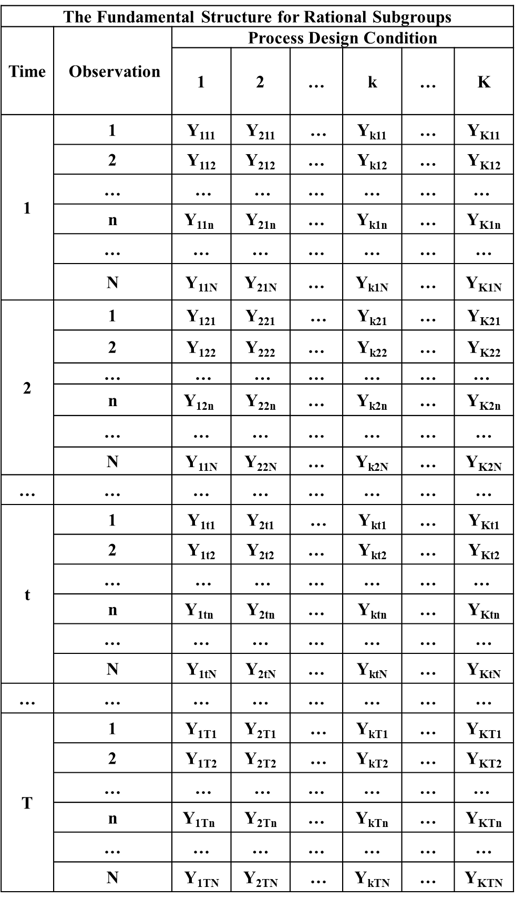
Figure 14-1. The Fundamental Rational Subgrouping Structure for VAS Data
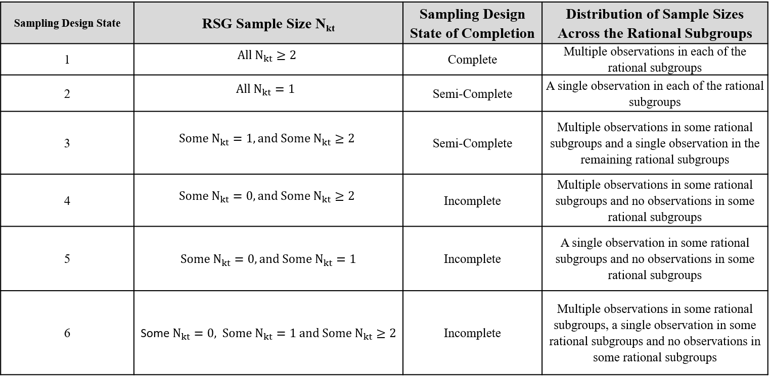
Table 14-1. The Six Sampling Design States
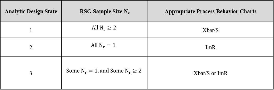
Table 14-2. The Three Analytic Design States
Equation 14-1. The Re-Parameterized Model Supporting the VAS Analyses
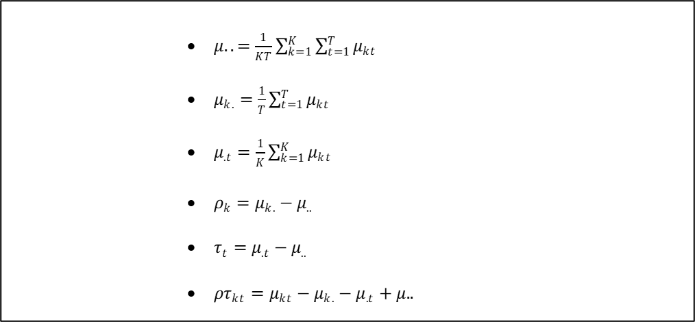
Figure 14-2. Re-Parameterized Model Parameter Definitions
The estimates of the fixed parameters in Equation 14-1 are presented in Figure 14-3 where
(A picture Word stores as a Windows metafile, image32.emf, which browsers cannot show; it will be converted.)
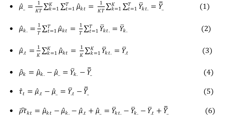
Figure 14-3. Estimated of the VAS Model Parameters
There are four classes of model components in Equation 14-1.
The process mean
The process design condition main effects
The production time main effects
The process design condition by production time interaction effects , and
The unexplained error terms .
Theoretically the first four groups involve parameters associated with “fixed” values. But the error terms are random variables whose values change across the observations. The error terms play a fundamentally different role in describing the behavior of the observed performance measurements because they are creating the unexplained variation or “noise” in the data obscuring the values of the fixed model parameters.
The VAS strategy is to re-create the model in Equation 14-1 by estimating the fixed model parameters as described above and “reconstructing” the model error terms. The reconstructed error terms are then superimposed back onto the estimates of the model parameters. The justification for this heuristic approach is that once the model is re-created, process behavior charts become a natural graphical analysis tool used to separate the signals in the data from the “unexplained” causes of variation. The estimation of the model parameters, and the reconstruction of the error terms, is accomplished through adjustments made to the original performance measurements which are referred to as the “R Residuals”.
14.1.1 Cautions Associated with Analyses Based on SDS = 4, 5 and 6
The VAS methodology is primarily directed at studies involving sampling design states 1 and 2, and sampling design state 4 when 4 is chosen by the analyst as part of a designed experiment or statistical process control system. Sampling design states 2 and 3 are semi-complete which creates problems in separating the PDCxPT interaction effects from the unexplained causes of variation.
Sampling design states 4, 5, and 6 are incomplete, and the data may be so sparse that significant biases and misleading information can be produced by the analyses. In some cases, the data may be so sparse as to make the analysis impossible. While VAS can handle these sampling design states the results must be viewed with caution.
14.2 The R1 Residuals – Centering the Original PM Data at 0
The first adjustment simply centers the original performance measurement data at 0 according to Equation 14-2.
Equation 14-2. The R1 Residuals
The R1 residuals are equivalent to the original performance measurement data . The information contained in the variation in the R1 residuals is identical to the information contained in the original measurements .
One use of the R1 residuals is to view the total range of variation in the original data as +/- limits about 0 as illustrated in Figure 14-4. But, the primary use of the R1 residuals is to analyze the behavior of the rational subgroup means and standard deviations across the process design condition by production time (PDCxPT) rational subgroups. In addition, the R1 residuals are used to analyze the behavior of the rational subgroup means and standard deviations across production time within each of the process design conditions.
14.2.1 The Rational Subgrouping Structure for the R1 Residuals
Since the R1 residuals are effectively the original performance measurement data simply centered near 0, the rational subgrouping structure for the R1 residuals is the same as the data presented in Figure 14-1.
14.2.2 Method of Analysis of the R1 Residuals
The primary use of the R1 residuals is the fundamental analysis of the behavior of the rational subgroup means and standard deviations across the R = KxT rational subgroups in Figure 14-1. This analysis provides information regarding the stability of the performance measure over both the process design conditions and production time.
The method of analysis of the R1 residuals depends upon the analytic design state for the rational subgrouping structure. For SDS = 1 and 4, the ADS = 1 so the Xbar/S charts are used. For SDS = 2 and 5 the analytic design state is ADS = 2 so the ImR charts are used to create the appropriate process behavior charts. For SDS = 3 and 6, the ADS = 3, and since for some of the rational subgroups, the default option in VAS is to use the Xbar/S charts in this scenario.[42]
The R1 residuals are centered at 0, but VAS allows the analyst to re-center the R1 residuals so that the Xbar and Individuals charts are on the same scale as the original performance measurements.
14.3 The R2 Residuals – Reconstruction of the Error Terms
Extracting the information related to the unexplained causes of variation from each of the original data points is an extremely important part of the VAS methodology. The algorithms required to reconstruct the error terms depend upon the sampling design state (SDS) associated with the rational subgrouping structure in Figure 14-1.
14.3.1 The Method of Calculating the R2 Residuals for SDS = 1 and SDS = 4
For sampling design states 1 and 4, the sample sizes are for each of the rational subgroups in Figure 14-1 that contain data (SDS 4 has for some rational subgroups). In this case the R2 residuals are calculated as in Equation 14-3.
Equation 14-3. The R2 Residuals for SDS 1 and SDS 4
14.3.2 The Rational Subgrouping Structure for the R2 Residuals for SDS 1 and 4
The rational subgrouping structure for the R2 residuals for SDS 1 and 4 is given in Figure 14-5. (Again, for SDS 4, the number of process design conditions will be less than K.)
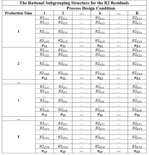
Figure 14-5. R2 RSB Structure for SDS 1 and 4
14.3.3 The Method of Analysis of the R2 Residuals for SDS 1 and 4
The sample sizes are for all of the rational subgroups Figure 14-5. Therefore the analytic design state is ADS 1 for both SDS 1 and SDS 4, and the S chart is used to analyze the data in this case.
14.3.4 The Method of Calculating the R2 Residuals for SDS = 2
When dealing with sampling design state 2 there is only a single observation in all of the rational subgroups in Figure 14-1. Attempting to reconstruct the R2 residuals using the method for SDS 1 using Equation 14-3 provides no information regarding the unexplained causes of variation since all of the R2 residuals equal 0 in that case. To circumvent this problem the model error terms are estimated using a two-step process.
Step 1: First, the original data are sorted by the K process design conditions and then by the T production times within each process design condition. Next the data are adjusted for the process mean, the process design condition main effects and the production time main effects as in Equation 14-4.
Equation 14-4. First Adjustment to the Data for ADS = 2
This is simply the PDCxPT interaction term which is exactly the error term used in general linear models with only a single observation in each treatment group.[43] But, if there is significant interaction between the process design conditions and production time, the variation in the is affected by the interaction terms and therefore exceeds the variation due to the error terms . This is the point where classical anova or general linear model methods stop and use the interaction terms as the “error” terms in the analysis. The VAS methodology goes one step further and adjusts the data by approximately removing the interaction effects. This approach makes the analysis of the process design conditions, process design factor effects, and production time main effects more sensitive, and it allows for the graphical analysis of the process design condition by production time interaction effects.
Step 2: The second step is a heuristic technique to remove the interaction effects from the data as follows. The sorted values are re-indexed where j = 1, 2,…, KT where KT is the total number of values.
Next the lagged values are calculated by
Equation 14-5. Lagged Z Values
The moving average (MA) of size 2 is calculated by using Equation 14-6.[44]
Equation 14-6. Moving Average for Lagged Z Values
The R2 residuals are then calculated using Equation 14-7.
Equation 14-7. R2 Residuals for SDS 2
where c(K,T) is the “rescaling” factor given in Equation 14-8.
Equation 14-8. R2 Rescaling Factor c(K,M)
14.3.5 The Rational Subgrouping Structure for the R2 Residuals for SDS 2
The rational subgrouping structure for the R2 residuals is presented in Figure 14-6Figure 14-7.
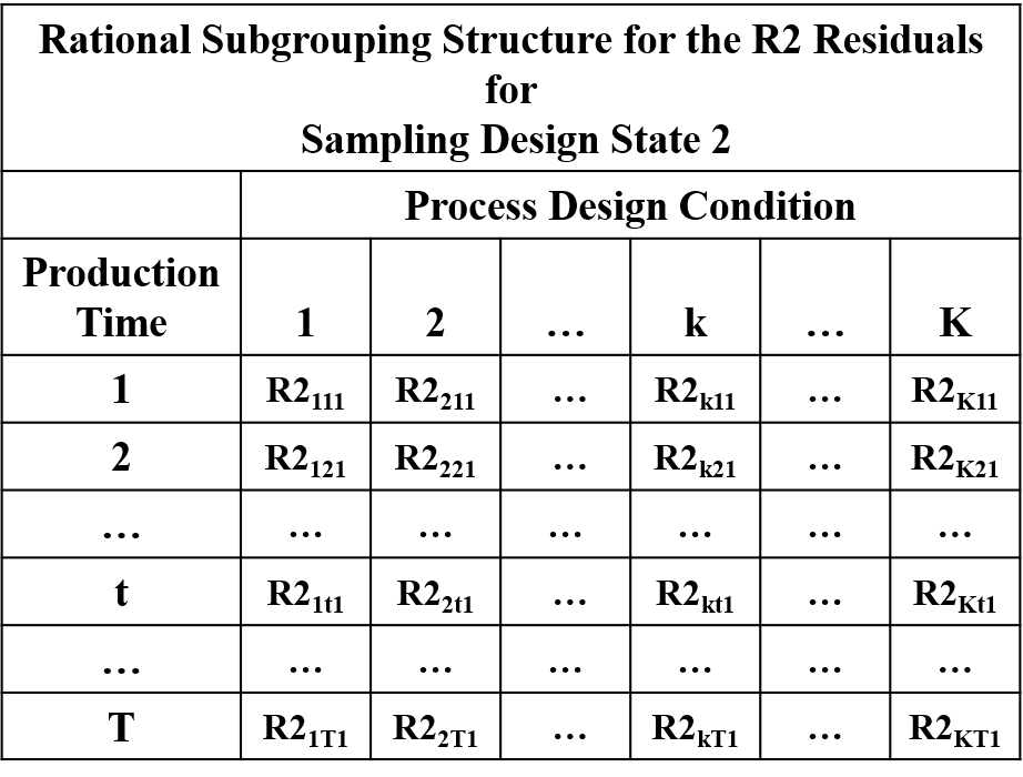
Figure 14-6. The RSG Structure for the R2 Residuals for SDS 2
14.3.6 Method of Analyzing the R2 Residuals for SDS 2
The sampling design state SDS 2 maps into the analytic design state ADS = 2. Therefore, the R2 residuals are analyzed using the moving range chart.
14.3.7 The Method of Calculating the R2 Residuals for SDS = 3, 5 and 6
The sampling design states 3, 5 and 6 have a single observation in some of the rational subgroups in Figure 14-1. Just as with SDS 2 attempting to reconstruct the R2 residuals using the method for SDS 1 provides no information regarding the unexplained causes of variation for those rational subgroups where . So in these cases VAS uses the same method for calculating the R2 residuals as for SDS 2 with only an adjustment made the rescaling factor c(K,T). The practical justification for this choice is that there can be many different levels of “sparseness” of the data (i.e. the percentage of rational subgroups where ). The method for ADS = 2 is designed to work for the case where all of the , and simulation studies show that this method works very well even for SDS = 1. Therefore, since the sample sizes in SDS 3, 5 and 6 are a combination of the sample sizes in SDS 1 and SDS 2, this approach should work well in many applications encountered in practice.
Step 1: First, the original data are sorted by the K process design conditions and then by the T production times within each process design condition. Next the data are adjusted for the process mean, the process design condition main effects and the production time main effects as in Equation 14-9.
Equation 14-9. First Adjustment to the Data for SDS = 3, 5 and 6
Step 2: The sorted values are re-indexed where j = 1, 2,…, M where M is the total number of values.
Next the lagged values are calculated as in Equation 14-10.
Equation 14-10. Lagged Z Values
The moving average (MA) of size 2 is calculated by using Equation 14-11Equation 14-6.
Equation 14-11. Moving Average for Lagged Z Values
The R2 residuals are then calculated using Equation 14-12Equation 14-7
Equation 14-12. R2 Residuals for SDS = 3, 5 and 6
where c(K,M) is given in Equation 14-13.
Equation 14-13. R2 Rescaling Factor c(K,M) for SDS 3, 5 and 6
14.3.8 The Rational Subgrouping Structure for the R2 Residuals for SDS 3, 5 and 6
The rational subgrouping structure for the R2 residuals for SDS 3, 5 and 6 is presented in Figure 14-7.
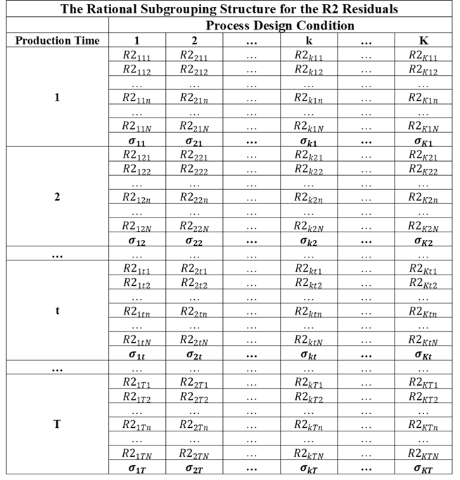
Figure 14-7. The RSG Structure for the R2 Residuals for SDS 3, 5 and 6
14.3.9 The Method of Analysis of the R2 Residuals for SDS 3, 5 and 6
The method of analysis for the R2 residuals depends upon the analytic design state for the rational subgrouping structure in Figure 14-7. For SDS = 5 for all of the rational subgroups containing data and so maps into ADS = 2. Therefore the moving range chart is used to analyze the R2 residuals for SDS 5. The sampling design states SDS 3 and SDS 6 map into ADS 3 and contain observations for some of the rational subgroups. Based on practical considerations, VAS defaults to the use of the S chart to analyze the R2 residuals in this case. If the data are very sparse, this will be evident on the S chart.[45]
14.4 The R3 Residuals – Analysis of the PDCxPT Interaction Effects
The data are next simultaneously adjusted for the process mean, the global process design condition effects and the global production time effects. These adjustments create the set of R3 residuals calculated as in Equation 14-14.
Equation 14-14. The R3 Residual Algorithm
The R3 residuals are modeled according to Equation 14-15.
Equation 14-15. The Model for the R3 Residuals
So the R3 residuals will be approximately free of any global process design condition effects and any global production time effects. These residuals will only be affected by assignable causes associated with the interaction effects , and by the unexplained model components , and the unexplainable model component . If the model parameters and are negligible, then
So in this case the R3 residuals provide information about the interaction between the process design conditions and production time.
14.4.1 The Rational Subgrouping Structure for the R3 Residuals
The rational subgrouping and statistical structure for the R3 residuals is presented in Figure 14-8.
14.4.2 The Method of Analysis of the R3 Residuals
As with the R2 residuals the method of analysis for the R3 residuals depends upon the analytic design state for the rational subgrouping structure in Figure 14-8. For ADS = 1 the sample size for all of the rational subgroups, so the Xbar/S charts are used to analyze the interaction effects. For ADS = 2 all of the rational subgroup sample sizes so the ImR charts are used to analyze the interaction effects. Again for practical reasons, for ADS = 3, the Xbar/S charts are used to analyze the R3 residuals.
14.5 The R4 Residuals – Analysis of the Production Time Effects
The original performance measurement data are next adjusted for the process mean, the global process design condition effects, and the process design condition by production time interaction effects as shown in Equation 14-16.
Equation 14-16. The R4 Residual Algorithm
The R4 residuals are modeled according to Equation 14-17.
Equation 14-17. The Model for the R4 Residuals
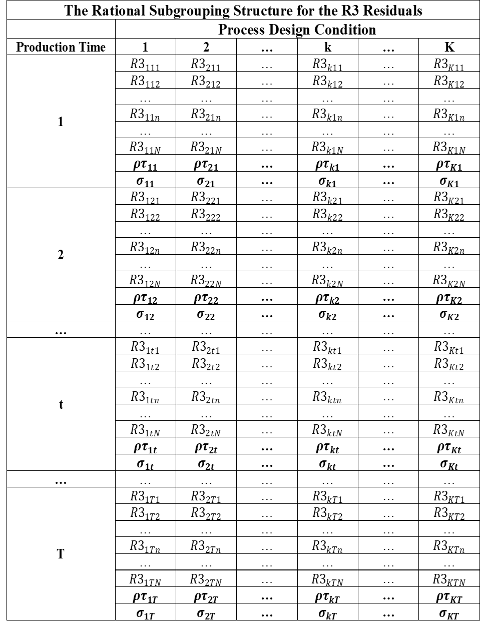
Figure 14-8. The RSG Structure for the R3 Residuals
From Equation 14-17 it can be seen that the R4 residuals are only affected by the assignable causes associated with the global production time effects and by the unexplained model components , and If the model parameters and are negligible, then
So in this case the R4 residuals provide information on the global production time effects .
14.5.1 The Rational Subgrouping Structure for the R4 Residuals
The rational subgrouping structure for the R4 residuals is presented in Figure 14-9. Note that while the rational subgroup sample sizes for the original R = KxT rational subgroups are , the rational subgroup sample size for the R4 residuals for production time t is always larger and given in Equation 14-18. Therefore the analytic design state for the R4 residuals will always be ADS = 1.
Equation 14-18. The Sample Size for the Production Time t RSG
14.5.2 The Method of Analysis of the R4 Residuals
Since ADS = 1 for the R4 residuals, the Xbar/S charts are used to analyze the R4 residuals which measure the global effects of production time on the performance measurement.[46]
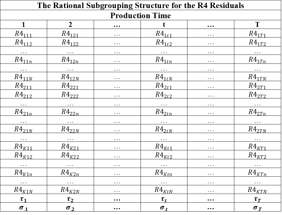
Figure 14-9. The RSG Structure for the R4 Residuals
14.6 The R5 Residuals – Analysis of the Process Design Condition Effects
The original performance measurement data are next adjusted for the process mean, the global production time effects, and the process design condition by production time interaction effects as shown in Equation 14-19.
Equation 14-19. The R5 Residual Algorithm
The R5 residuals are modeled as in Equation 14-20.
Equation 14-20. The Model for the R5 Residuals
If the model parameters and are negligible, then
So in this case the R5 residuals provide information on the global process design condition effects .
14.6.1 The Rational Subgrouping Structure for the R5 Residuals
The rational subgrouping structure for the R5 residuals is presented in Figure 14-10. Note again that while the rational subgroup sample sizes for the original R = KxT rational subgroups are , the rational subgroup sample size for the R5 residuals for process condition k is always larger and given in Equation 14-21. Therefore the analytic design state for the R5 residuals will always be ADS = 1.
Equation 14-21. The Sample Size for the Process Design Condition k RSG
14.6.2 The Method of Analysis of the R5 Residuals
Since ADS = 1 for the R5 residuals, the Xbar/S charts are used to analyze the R5 residuals which measure the global effects of the process design conditions on the performance measurement.
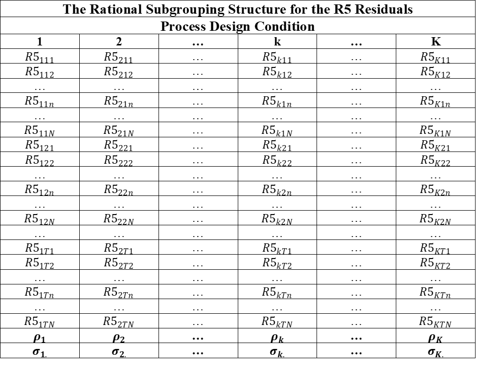
Figure 14-10. The RSG Structure for the R5 Residuals
14.7 The R6 Residuals – Analysis of the Process Design Factor Main Effects
The R5 residuals contain all of the available information about the process design conditions , and therefore the process design factor effects. When there are multiple process design factors creating the process design conditions, the PDC effects can be decomposed into the contributions due to the main effects and interaction effects of the process design factors.
As an example of the decomposition of the process design condition parameters consider the case where there are two process design factors occurring at I levels and occurring at J levels. In this case the K process design conditions are created by the combinations of the I levels of factor and the J levels of factor . The process design condition effects can be written as
Equation 14-22. The PDC Effects as a Function of the Process Design Factor Effects
with the additional constraints
Equation 14-23. The Constrains of the Process Design Factor Effects
The parameters and are the main effects for Factor 1, the main effects for Factor 2 and the Factor 1 by Factor 2 interaction effects respectively.
When there are a large number of process design factors the analysis of the interactions becomes cumbersome because of the large number of interaction effects. For example, if we have M=6 process design factors, then there are 15 two-factor interactions, 20 three-factor interactions, 15 four factor interactions and 6 five factor interactions. Three-factor interactions and above are often difficult to interpret, and fortunately in many applications it is found that these higher order interactions are not of practical significance.[47] Therefore VAS restricts the analysis of the effects of multiple process design factors to their main effects.
The process design factor main effects can be estimated using the R5 residuals in the following way. Consider the case where there are M process design factors , and factor occurs at I levels i = 1,2, …,I. The main effect for the ith level of factor is given by Equation 14-24 where average of the R5 residuals for the ith level of factor .
Equation 14-24. Process Design Factor Main Effect Estimate
The factor main effects are analyzed by creating the R6 residuals as in Equation 14-25.
Equation 14-25. The Algorithm for Calculating the R6 Residuals
14.7.1 The Rational Subgrouping Structure for the R6 Residuals
The rational subgrouping for the analysis of the main effects for the process design factors is presented in Figure 14-11.
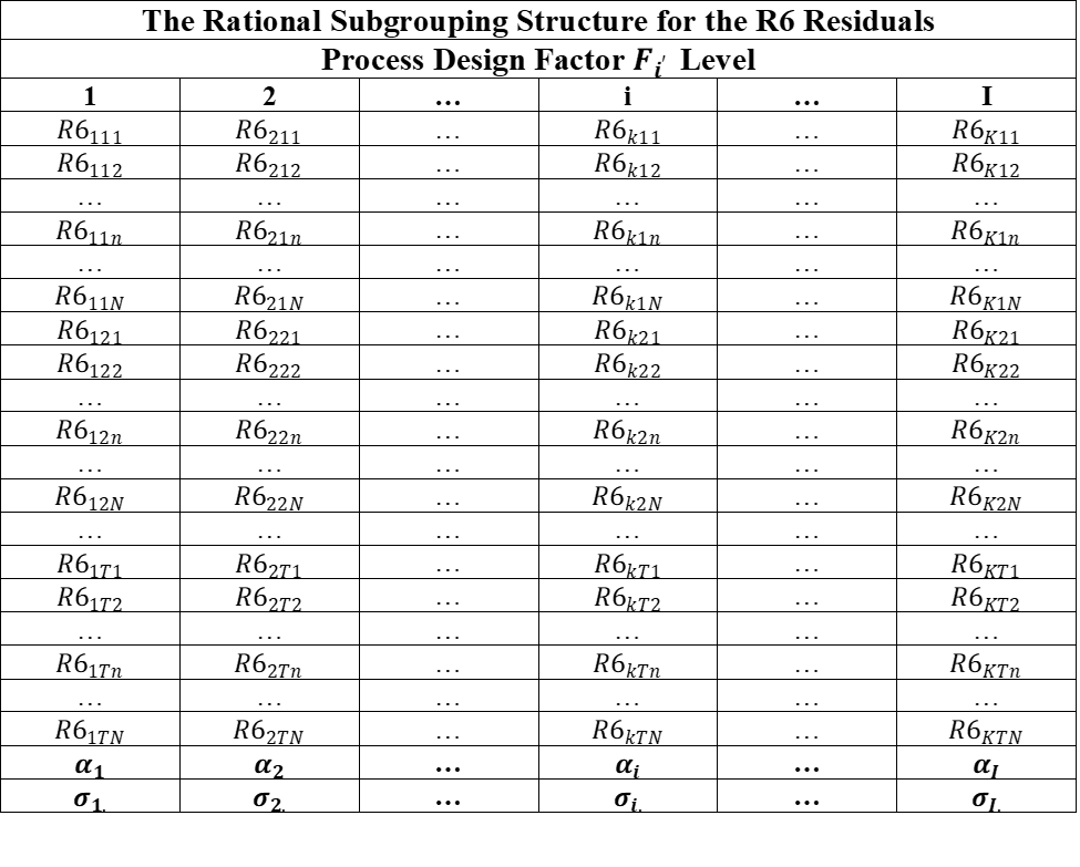
Figure 14-11. The RSG Structure for the R6 Residuals
14.7.2 The Method of Analysis of the R6 Residuals
The analytic design state for the rational subgrouping structure in Figure 14-11 will always be ADS = 1. Therefore, the Xbar/S charts are used to analyze the R6 residuals which measure the main effects of the process design factors on the performance measurement.
14.8 Re-Centering the R Residuals
The R residuals are all centered at or near 0 which is often convenient because the Xbar and Individual process behavior charts are centered at 0. In this case the behavior charts provide the analyst with direct information on the size of the effects being analyzed in terms of +/- limits about 0. But in some cases the analyst wants to analyze the R residuals and interpret the results on the original scale of measurement. In this case re-centering the R residuals at the overall average value for the performance measurement accomplishes this goal. So VAS allows the analyst to base the analyses on the re-centered R1, R3, R4, R5 and R6 residuals calculated using Equation 14-26.
Equation 14-26. The Re-Centered R Residuals
It is incumbent on the analyst to study and understand the sparseness of the data used in these analyses.
Note: See Chapter 19 of Applied Linear Statistical Models by Neter and Wasserman (1974).
There are a number of methods for fitting smooth curves through data. The method presented has been chosen on the basis of its simplicity, and the fact that it works well in practice.
Again, it is incumbent on the analyst to understand the sparseness of the data.
The only time this condition could be violated is in the case where the data are so extremely sparse that the analysis is a moot point.
See the note on page 646 of Applied Linear Statistical Models by Neter and Wasserman where they address this issue.