19.0 The Analysis of Cup Fill Weights
Part IX. An Example of VAS Analyses
There is an extensive amount of research that is conducted by analysts and engineers in industrial environments in order to “optimize” the performance of manufacturing processes. Many consumer product companies use high speed filling machines to place their product into containers. In this application a homogeneous product similar to yogurt is filled into plastic cups. One of the primary goals is minimizing the cost of raw materials used in the production process while at the same time ensuring that all cups meet the label claim of 232 grams. The way to meet these two requirements is to understand, control and possibly reduce the variation in the fill weights.
19.1 The Specification Limits
Specification limits or standards define the acceptable range for process variation. In this case the label claim of 232 grams was a mandated lower bound for the fill weights. Based on an economic analysis it was determined that any cup fill weight above 242 grams was an unacceptable waste of raw materials. These conditions led the following specification limits.
Lower Specification Limit (LSL) = 232 Grams
Target Value (TV) = 237 Grams
Upper Specification Limit (USL) = 242 Grams
19.2 Analysis of the Process Design
The first step in the analysis of the variation in the cup fill weights was the creation of the process design diagram presented in Figure 19-1.
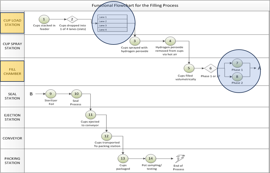
Figure 19-1. The Process Design Diagram for the Cup Filling Process
From that diagram we see that there are 4 parallel “Filling Lanes”, so 4 cups are simultaneously filled at any point in time. In addition, we see that each lane is associated with a filling chamber. Each filling chamber used a cylinder of known volume and a piston inside the cylinder as illustrated in Figure 19-2.
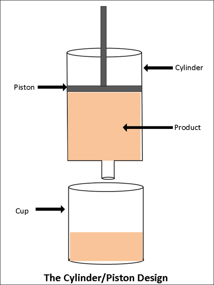
Figure 19-2. The Design of the Pistons Associated with the Filling Chambers
As the piston is raised within the cylinder the product is introduced into the cylinder from the bottom and an empty cup is simultaneously indexed under the cylinder filling head. Once the piston reaches the top of the cylinder there is a known volume and, assuming constant product density, a known weight of product in the cylinder. The next step in the process is to push the piston down which forces the product from the cylinder into the cup. As the piston is moving down the cylinder is refilled from the top. As the piston is brought back up the next cup is filled and the cylinder is refilled from the bottom. So in this design a cup is filled on each up and down stroke of the piston. These two stokes of the piston were referred to as “Phase 1” and “Phase 2” as illustrated in Figure 19-1. So the analysis of the process design identified two process design factors “Lane” at 4 levels and “Phase” at 2 levels. These two factors combined to form a total of 8 “process design conditions”.
19.3 The Sampling Plan and Rational Subgrouping Structure
A study was conducted in which a sample of N=5 cups was selected from the process for each of the 8 process design conditions for each of T=100 consecutive production times. This sampling plan led to the rational subgrouping structure presented in Figure 19-3 where N = 5 and T = 100 for a total of 4000 observations. A partial list of the data is presented in Table 19-1.
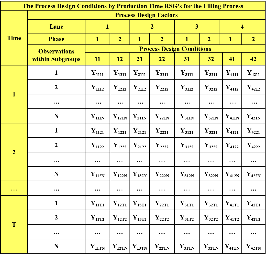
Figure 19-3. Rational Subgrouping Structure for the Fill Weight Study
Table 19-1. Partial List of the Fill Weight Data
19.4 Input to “Process Behavior” Software
In order to analyze the variation in the cup fill weights using the Process Behavior library, we only need to import the data file, input the following information and direct the system to “formulate” the problem. Once this is accomplished the Process Behavior software produces a set of graphical output that is used to analyze the variation observed in the fill weights.
The performance measurement – Fill Weight
The process design factors:
a. Factor 1 – Lane
b. Factor 2 – Phase
The production time variable – Pull
The specification limits.
19.5 Output Produced by the Process Behavior Software
The following graphical output is partial list of the analyses produced by the Process Behavior software. A brief description of the information contained in the graphs is provided.
From Figure 19-4 it is clear that the current variation in the fill weights is too large to consistently satisfy the specification limits. Approximately .45% of cups are filled below the lower specification limit and .53% are filled above the upper specification limit. The overall standard deviation is estimated to be 1.74 grams.
The questions of interest now related to the “causes” of this variation and the relative contribution of the causes to the total variation observed in the fill weights. Figure 19-5 and Figure 19-6 are the process behavior charts for the PDCxPT rational subgroup sample means and standard deviations based on the rational subgrouping structure in Figure 19-3. The Xbar chart for the sample means demonstrates that the variation in the sample averages is “uncontrolled” across the rational subgroups indicating that either the process design conditions and/or production time are associated with assignable causes creating nonrandom variation in the fill weight averages.
The S chart for the rational subgroup standard deviations demonstrates that the variation within the rational subgroups is relatively “controlled” near 1 gram.
The next step in the analysis is to analyze the variation in fill weights across production time within each of the 8 process design conditions. Figure 19-7 through Figure 19-10 are examples of the information produced by these behavior charts for the Lane 4-Phase 1 and Lane 4-Phase 2 process design conditions. It can be seen from Figure 19-7 that the variation in the average fill weights over time for Lane 4 – Phase 1 is uncontrolled with obvious “jumps” in the fill weights. Figure 19-9 is the companion chart for Lane 4 – Phase 2, and it can be seen that similar “jumps” are occurring, but in the opposite direction. This indicates that the fill weights for Lane 4 - Phase 1 and Lane 4 – Phase 2 are “negatively correlated”. That is, these two process design conditions are “stealing” from each other. When Lane 4 – Phase 1 over fills a cup, Lane 4 – Phase 2 under fills a cup. This negative correlation is significantly increasing the total variation in fill weights.
The S charts in Figure 19-8 and Figure 19-10 indicate that the standard deviations are controlled across production time near an average of 1 gram.
Figure 19-7. Analysis of Effect Time on the Sample Means for PDC 4-1
Figure 19-8. Analysis of the Effect of Time on the Standard Deviation for PDC = 4-1
Figure 19-9. Analysis of the Effect of Time on the Sample Means for PDC = 4-2
Figure 19-10. Analysis of the Effect of Time on the Standard Deviation for PDC = 4-2
Figure 19-11 and Figure 19-12 present the analysis of the main effects of the 8 process design conditions. Figure 19-11 clearly demonstrates that there are assignable causes of variation associated with the lanes and phases. Phase 2 is producing higher average fill weights within all four lanes which is an example of the principle of the “nontrivial replication of results”. Lane 3 appears to be producing lower average fill weights compared to the other three lanes.
Figure 19-12 again demonstrates that the standard deviations are comparable across the 8 process design conditions.
Figure 19-12. Analysis of Effect of PDC on Sample Standard Deviations
The Process Behavior software then produces “main effects” charts for the process design factors Lane and Phase. These analyses are presented in
Figure 19-14. Analysis of the Lane Effect on the Sample Standard Deviations
Figure 19-16. Analysis of the Phase Effect on the Sample Standard Deviation
The system next produces an analysis of the effects of production time on the variation in fill weights. Figure 19-17 indicates that the variation in the average fill weights across production time is relatively stable or controlled. Similarly, Figure 19-18 indicates that the standard deviations are relatively stable or controlled across production times.
Figure 19-17. Analysis of Production Time Effect on the Sample Averages
Figure 19-18. Analysis of the Production Time Effects on the Sample Standard Deviations
At this point Process Behavior system has identified the fact that there are assignable causes of variation associated with the factors Lane and Phase that are affecting the variation in the fill weights. The Process Behavior system then produces the Taguchi loss function analysis presented in Figure 19-19. This chart indicates that only about 21% of the loss associated with the observed variation in fill weights is due to “unexplained” causes of variation. The most significant contribution to the observed variation is associated with the process design condition by production time interaction. This accounts for 44.5% of the loss, and is due to the “jumps” in fill weights over time within the 8 lane-phase process design conditions. Approximately 13% of the variation is due to the main effects of lane and phase shifting the process mean systematically away from the target value. In addition, approximately 17% of the loss is due to the overall process average being shifted away from the target value of 237 grams. Production time does not appear to have any practical effect on the variation in the fill weights.
The final step in the analysis is the determination of how much the variation in fill weights would be reduced if actions could be taken to remove the assignable causes identified as creating nonrandom variation in the fill weights. Figure 19-20 presents these results which indicate:
The overall standard deviation can potentially be reduced from 1.74 grams to .80 grams
The filling process would be more than capable of meeting the specification limits.
19.6 Epilogue
As a final note related to this case study, the process engineers were able to discover the primary cause producing the assignable causes detected by the Process Behavior analyses. It was due to a pump inside a “surge tank” controlling the flow of product from the manufacturing plant to the filling machine. The filling process was re-engineered and the surge tank was removed. The variation in the cup fill weights for the re-designed process then matched Figure 19-20.