21.0 Statistical Process Control Applications
The analytical capabilities of Process Behavior also extend to statistical process control applications.[54] In order to illustrate this we apply the capabilities of Process Behavior to two examples presented in Dr. Wheeler’s book Understanding Statistical Process Control.
21.1 Analysis of Wheeler Part Thickness Data - Example 3.1
Consider the analysis of the 80 measurements presented in Table 21-1 which are the data associated with Wheeler’s example 3.1. which are part thicknesses measured in amounts that exceeded 0.300 inches, in units of one-thousandth of an inch. The Xbar/S process behavior charts are presented in Figure 21-1 and Figure 21-2 which match Wheeler’s results.[55]
Table 21-1. Part Thickness Data
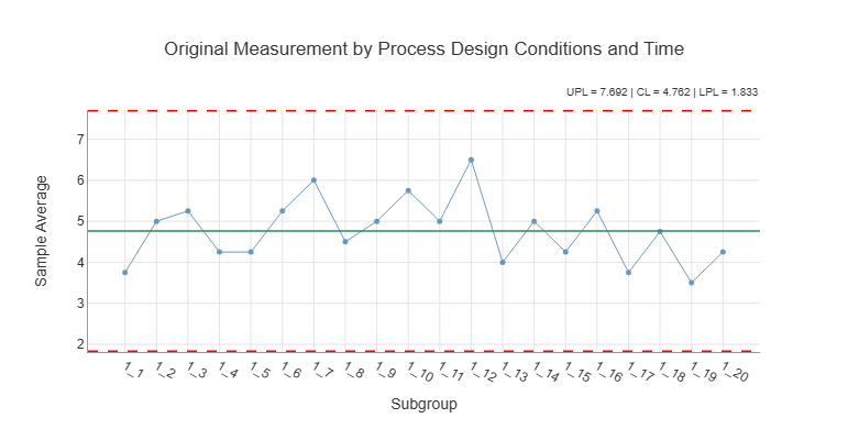
Figure 21-1. Xbar Chart Over Production Time
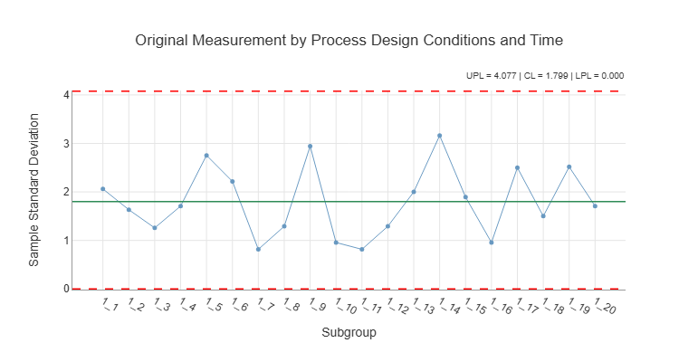
Figure 21-2. S Chart Over Production Time
21.2 Analysis of Ball Socket Joint Data - Wheeler Example 6.1[56]
A certain type of ball joint socket is manufactured using an injection molding process. The process was designed using 4 “cavities” so 4 ball joints were produced at each point in time. The response variable was “socket thickness” in excess of 12.00 millimeters measured in hundredths of a millimeter. The specification limits were LSL = 0 and USL = 15 hundredths of a millimeter. The data for 24 consecutive sample pulls from the process are presented in Table 21-2.
Table 21-2. Wheeler Ball Socket Data
The data were analyzed by Process Behavior using Cavity as the process design factor at 4 levels. Remember the analysis is an inductive process so different analysts may conduct the analysis in different orders than presented here. The first step in the analysis was to assess the current process capability. This analysis is presented in Figure 21-3.
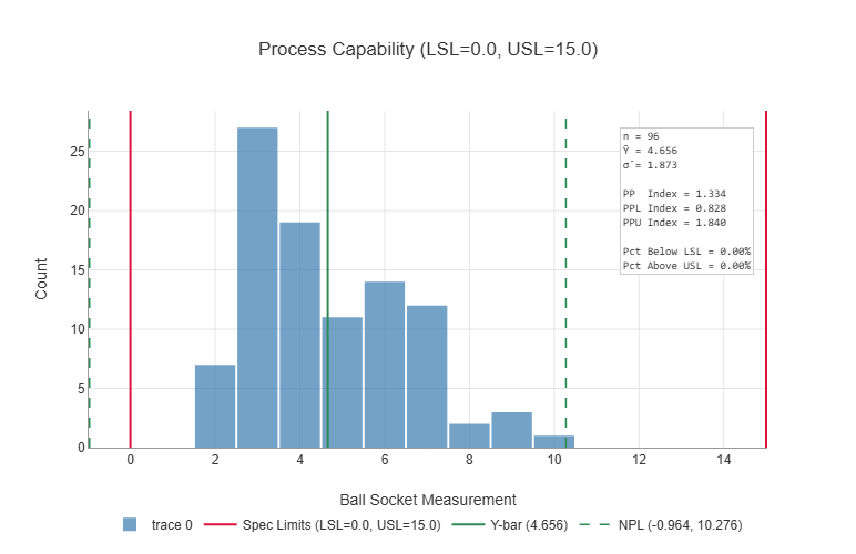
Figure 21-3. Current Process Capability
It can be seen from Figure 21-3 that the process produced all of the test data within the specification limits, but the PPL capability index is below 1 which means the process has the potential to produce product below the lower specification limit so a more detailed analysis of the causes of variation in the socket thickness is warranted.
Figure 21-4 displays some evidence that Cavity II is producing higher socket thickness values than the other 3 cavities. Figure 21-5 indicates that the standard deviations are in relatively good control and similar across the 4 cavities.
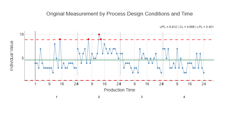
Figure 21-4. Individuals Chart for Socket Thickness by PDCxPT
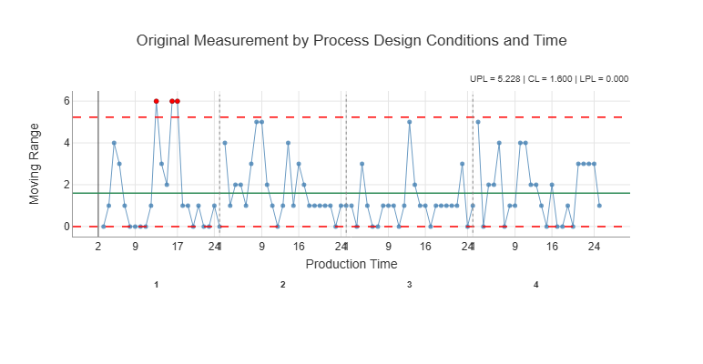
Figure 21-5. Moving Range Chart for Socket Thickness by PDCxPT
In order to pursue the cavity effects in more detail, the main effects analyses were reviewed. Figure 21-6 clearly indicates that there is a cavity effect on the average socket thickness with Cavity II producing higher measurements compared to the other three cavities. The review of Figure 21-7 indicates that there are no significant differences in the standard deviations across the cavities.
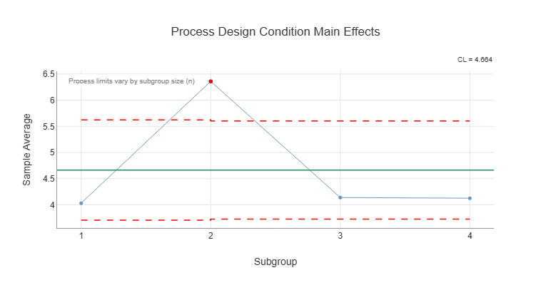
Figure 21-6. Main Effects Analysis for Cavities
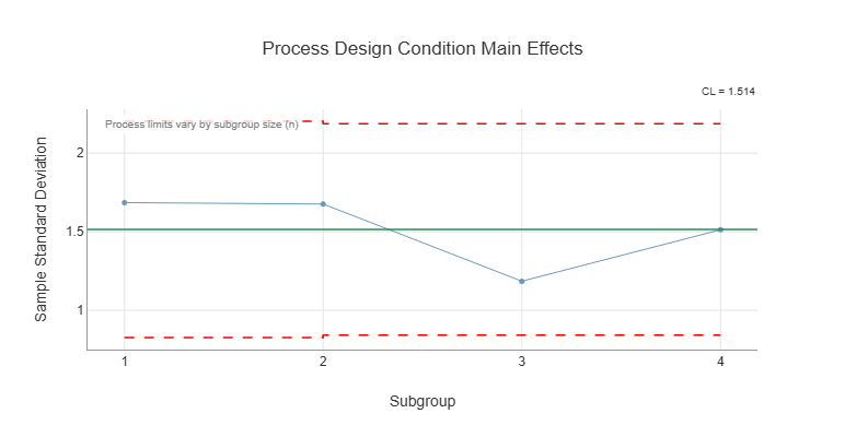
Figure 21-7. Analysis of Standard Deviations Across the Cavities
Next the stability of the process across production times was analyzed. Both Figure 21-8 and Figure 21-9 indicate the process is relatively stable across production runs with respect to both the subgroup means and standard deviations.
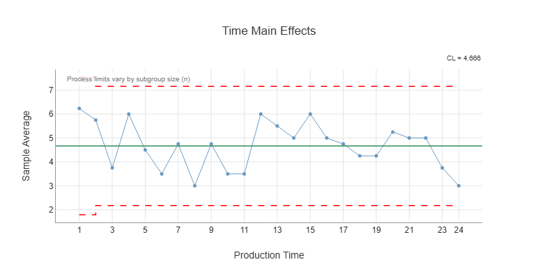
Figure 21-8. Main Effects Analysis for Production Time
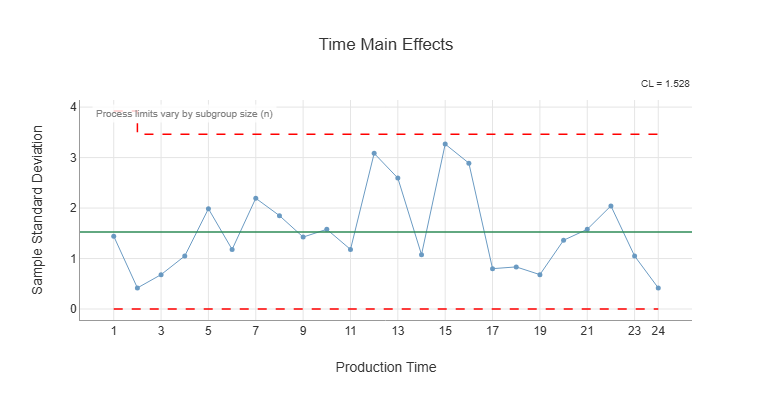
Figure 21-9. Analysis of Standard Deviations Across Production Time
Figure 21-10 and Figure 21-11 indicate that there is no significant interaction between the cavities and production time. Therefore, we conclude that the primary effect discovered over and above the unexplained causes of variation is the effect due to Cavity II on the average socket joint measurement.
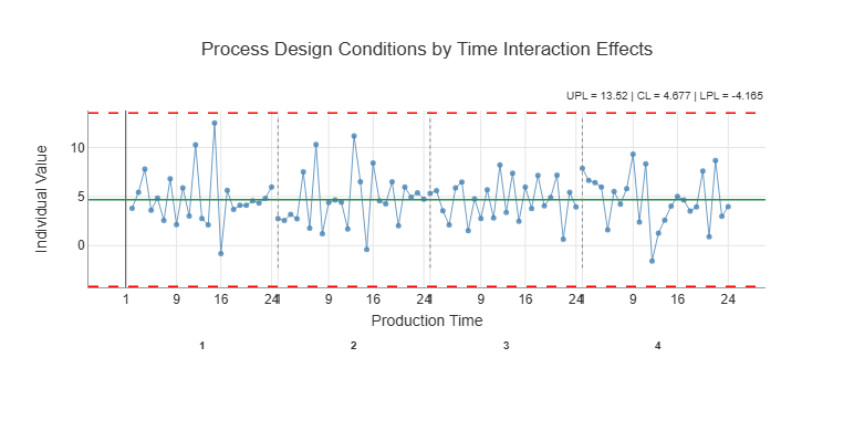
Figure 21-10. Interaction Effects for Cavity by Production Time
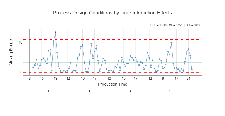
Figure 21-11. Standard Deviations for Interaction Effects
The Taguchi loss function presented in Figure 21-12 is helpful in assessing how much this discovered main effect of cavities has on the variation in the socket measurements. It can be seen from that figure that the cavities (PDC) are only contributing about 24% to the total loss. In addition the production time is contributing about the same amount and no significant effects of production time were discovered by the analysis. Therefore, the effect of removing the cavity effects will probably not improve the capability of the process to any great degree.
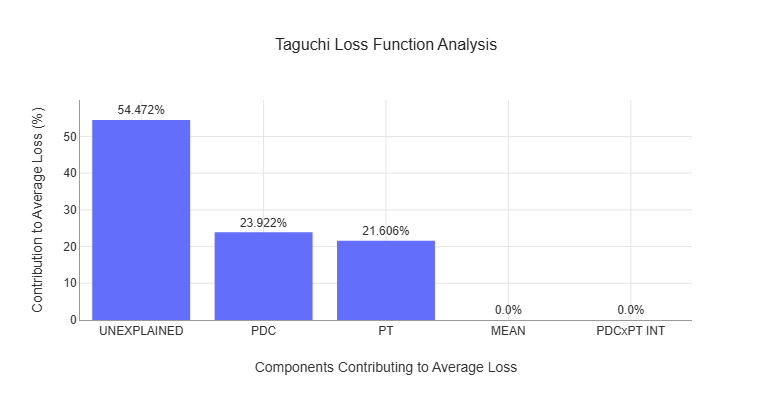
Figure 21-12. The Taguchi Loss Function Analysis for the Socket Measurements
Figure 21-13 presents the potential capability analysis that estimates how much the process capability would improve if Cavity II could be brought in line with the other three cavities. The lower capability index would approximately increase from 0.83 to 1.03 which is helpful, but the process would still be at risk of producing socket measurements below the lower specification limit.
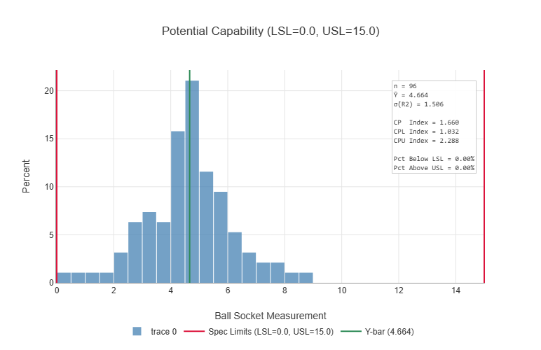
Figure 21-13. Potential Capability of the Socket Process
See Understanding Statistical Process Control” by Donald Wheeler for a detailed discussion of statistical process control concepts and strategies.
Note: The behavior limits do not match exactly because Wheeler uses the range chart to analyze these data in his Example 3.2.
See page 102 of Understanding Statistical Process Control for a complete description of this example.