12.0 The Individual and Moving Range Charts

There are many applications where there is only a single or individual measurement in each rational subgroup. This often results when a single measurement is obtained across some ordered sequence usually associate with time or space (so we are changing the subscript from r to t to reinforce this fact). The rational subgrouping structure in this case is presented in Figure 12-1.

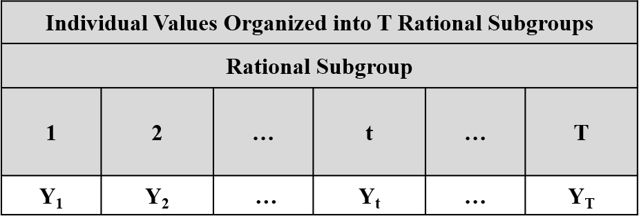
Figure 12-1. Rational Subgrouping Structure for Individual Values — **Figure 12-1.** Rational Subgrouping Structure for Individual Values

The question is how to extract out the information about the “unexplained” causes of variation in this case? Remember, assignable causes of variation produce nonrandom patterns of variation. Figure 12-2 is an example of data affected by a linear trend. Where is the “unexplained” variation in the data in Figure 12-2? It is in the variation of the individual values around the trend line as illustrated in Figure 12-3. Figure 12-4 provides an example of the case where there is a non-linear trend in the data. Again the unexplained variation is in the individual values about the non-linear trend. In these cases we must turn to the Individual-Moving Range (I-mR) charts for the analysis of the data.

Source:

Generated figures

Figure 12-2. Example of a Positive Linear Trend

Source:

Generated figures

Figure 12-3. The Unexplained Variation About a Linear Trend Line

Source:

Generated figures

Figure 12-4. The Unexplained Variation About a Non-Linear Trend Line

Now, if the samples are selected relatively close in time, then successive values of the performance measurement are logically comparable in that they are affected by the nonrandom trend in almost the same way.^[41] Therefore, the differences in successive values are basically unaffected by the nonrandom trend. That is, the variation in the differences in successive values of the performance measurement is due mostly to the unexplained causes of variation affecting the data. So the successive values $\left\{ Y_{t},Y_{t + 1} \right\}$ of the performance measurement constitute a series of “pseudo-samples” of size N=2 produced under “essentially the same conditions”. Now consider the successive moving ranges of order 2 defined by

{mR}_{2} = \left| Y_{2} - Y_{1} \right|

{mR}_{3} = \left| Y_{3} - Y_{2} \right|

...

{mR}_{T} = \left| Y_{T} - Y_{\ T - 1} \right|

The “average moving-range” is defined in Equation 12-1.

\overline{mR} = \ \frac{{mR}_{2} + {mR}_{3} + \ldots + {mR}_{T}}{T - 1} \tag{12-1}

Equation 12-1. The Average Moving Range

Now it is known that if $\left\{ Y_{1},Y_{2} \right\}$ is a random sample of size N=2 from a normal distribution with standard deviation σ, then the mean and the standard deviation for the range $R = \left| Y_{1} - Y_{2} \right|$ are given by Equation 12-2. These theoretical results form the basis for the construction of the ImR charts.

E(R) = \ \mu_{R} = 1.128\sigma\ \ and\ \ \ \sigma_{R} = .8525\sigma \tag{12-2}

Equation 12-2. The Mean and Standard Deviation for the Range

12.1 The Moving Range Chart¶

In this case we start the analysis by assuming that the rational subgroups are inert (i.e. they have no effect on the mean or standard deviation for the performance measurement Y. That is, the data $\left\{ Y_{1},Y_{2},\ldots,Y_{T} \right\}$ have been produced under essentially the same conditions. Under this assumption we can apply Chebyshev’s theorem and predict that at least 89% of the moving ranges $\left\{ {mR}_{t} \right\}$ should fall in the interval given in Equation 12-3.

\left\{ 1.128\sigma - 3(.8525)\sigma,\ 1.128\sigma + 3(.8525)\sigma \right\} = \ \left\{ 0,\ 3.686\sigma \right\} \tag{12-3}

Equation 12-3. The Three Sigma Limits for Moving Range

Again the parameter σ is unknown and must be estimated from the data. We use the estimate in Equation 12-4.

\widehat{\sigma} = \frac{\overline{mR}}{1.128} \tag{12-4}

Equation 12-4. The Estimate of σ Based on the Moving Range

It should be approximately the case that 89% of the moving ranges fall in the interval

\left\{ 0,\ 3.686\ \widehat{\sigma} \right\} = \left\{ 0,\ 3.686\frac{\overline{mR}}{1.128} \right\} = \left\{ 0,\ 3.268\ \overline{mR} \right\} \tag{12-5}

Equation 12-5. The Estimated Three Sigma Limits for the Moving Range

The moving ranges are plotted on an X-Y graph where the x-axis is the rational subgroup and the y-axis is the moving range. The centerline and the behavior limits are then superimposed on the X-Y graph.

If the assumption that the rational subgroups are inert is correct, or the successive values $\left\{ Y_{t},Y_{t + 1} \right\}$ of the performance measurement constitute a series of “pseudo-samples” of size N=2 produced under “essentially the same conditions”, then the moving ranges should vary randomly about the centerline within the behavior limits. The graph is analyzed for the presence of nonrandom patterns occurring across the rational subgroups that would indicate that the rational subgroups do, in fact, have an effect on the rational subgroup standard deviations.

12.2 The Individual Chart¶

Under the same assumptions forming the foundation for the analysis of the moving range, we can apply Chebyshev’s theorem and predict that at least 89% of the individual observations should fall within the interval given in Equation 12-6.

\left\{ \mu - 3\sigma,\ \mu + 3\sigma \right\} \tag{12-6}

Equation 12-6. The Three Sigma Limits for Individual Values

Again, the values for µ and σ must be estimated from the data. The estimate of the mean µ is given in Equation 12-7.

\widehat{\mu} = \overline{Y} = \ \frac{Y_{1} + Y_{2} + \ldots + Y_{T}}{T}\ . \tag{12-7}

Equation 12-7. The Estimate of the Mean for the Individual Chart

The standard deviation σ is estimated as in Equation 12-8.

\widehat{\sigma} = \frac{\overline{mR}}{1.128} \tag{12-8}

Equation 12-8. The Estimate of the Standard Deviation for the Individual Chart

The centerline for the Individual chart is given by Equation 12-9.

CL = \overline{Y} \tag{12-9}

Equation 12-9. The Centerline for the Individual Chart

The lower behavior limit for the Individual Chart is given by Equation 12-10.

LBL(Y) = \ \overline{Y} - 3\frac{\overline{mR}}{1.128} = \overline{Y} - 2.66\ \overline{mR} \tag{12-10}

Equation 12-10. The Lower Behavior Limit for the Individual Chart

The upper behavior limit for the Individual Chart is given by Equation 12-11.

UBL(Y) = \ \overline{Y} + 3\frac{\overline{mR}}{1.128} = \overline{Y} + 2.66\ \overline{mR} \tag{12-11}

Equation 12-11. The Upper Behavior Limit for the Individual Chart

The individual values Y are plotted on an X-Y graph where the x-axis is the rational subgroup and the y-axis is the individual value Y. The centerline and the behavior limits are then superimposed on the X-Y graph.

If our assumptions are correct, the individual values should vary randomly about the centerline within the behavior limits. The graph is analyzed for the presence of nonrandom patterns occurring across the rational subgroups that would indicate that the rational subgroups do, in fact, have an effect on the rational subgroup means.

Examples of the ImR charts are presented in Figure 12-5 and Figure 12-6.

Source:

Generated figures

Figure 12-5. Moving Range Chart for Y

Source:

Generated figures

Figure 12-6. Individual Chart for Y

12.3 The Choice for the Multiplying Factor - p¶

As with the Xbar and S charts, the multiplier 3 in the formulas for the process behavior limits can be adjusted by the analyst to change the sensitivity of the analyses. Again, if there is no compelling reason to make this change, it is recommended that Shewhart’s choice of p=3 be used to construct the charts.

Footnotes¶

How close is close depends upon the application and is determined during the problem formulation.
↩