11.0 The Xbar and S Charts - VAS Documentation Manual

Part VI. Shewhart Process Behavior Charts

The Shewhart process behavior charts are the primary graphical tools used within VAS to analyze data organized into various rational subgrouping structures to assess the effects of the process design conditions, process design factors and production time on the performance measurement of interest. The four types of process behavior charts used in VAS are the Xbar-S charts and the Individual-Moving Range charts. The details of the applications of these charts within VAS are presented in later chapters. But first, in this chapter and the next, we present the general logic and steps associated with the creation of these four process behavior charts.^[36]

11.1 The Generic Structure for Rational Subgroups¶

In previous chapters we introduced specific rational subgrouping structures related to the formulation of analytic studies. But process behavior charts are very flexible, and they can be created in a number of ways to answer specific questions about the cause system of variation under study. VAS takes advantage of this flexibility and uses a number of different rational subgrouping structures. So, at this point, we present the theory for the generic rational subgrouping structure associated with R subgroups and $N_{r}$ observations in the r^th rational subgroup as illustrated in Figure 11-1.

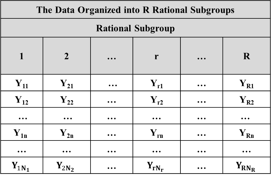
Figure 11-1. The Generic Structure of Data Organized into R Rational Subgroups — **Figure 11-1.** The Generic Structure of Data Organized into R Rational Subgroups

Under the assumption that the data have been produced by a constant cause system of variation, the statistical properties of the data are presented in Figure 11-2. The rational subgroup sample averages $\left\{ {\overline{Y}}_{r} \right\}$ and sample standard deviations $\left\{ {\overline{S}}_{r} \right\}$ are used to estimate the rational subgroup means $\left\{ \mu_{r} \right\}$ and standard deviations $\left\{ \sigma_{r} \right\}$ as illustrated in Figure 11-3.

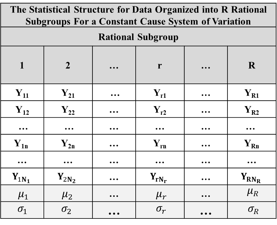
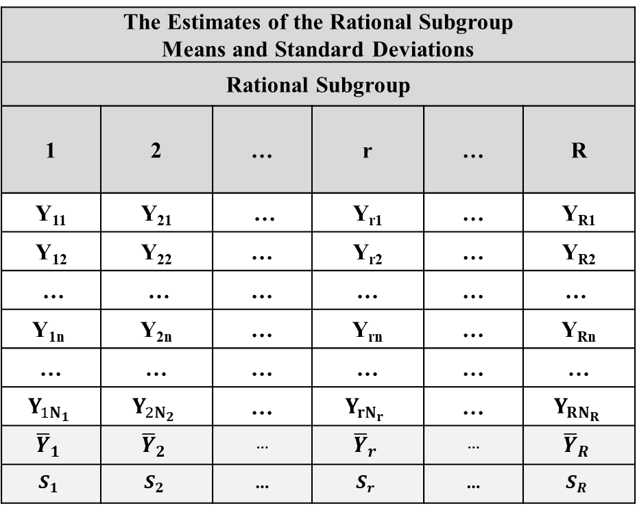
Figure 11-2. The Statistical Properties Associated with R Rational Subgroups — **Figure 11-2.** The Statistical Properties Associated with R Rational Subgroups

Figure 11-3. Estimates of the Rational Subgroup Means and Standard Deviations — **Figure 11-3.** Estimates of the Rational Subgroup Means and Standard Deviations

The analysis begins by making the initial assumption that the rational subgroups are “inert” meaning they have no effect on the rational subgroup means or standard deviations so the data within all of the rational subgroups have been produced “under essentially the same conditions”. Under this assumption the mean µ and the standard deviation σ are common to all of the rational subgroups so the statistical structure for the rational subgroups is that presented in Figure 11-4.

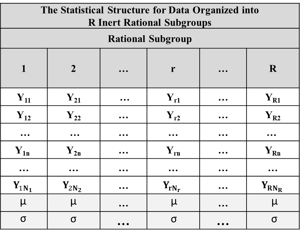
Figure 11-4. The Statistical Properties of the Data for Inert Rational Subgroups — **Figure 11-4.** The Statistical Properties of the Data for Inert Rational Subgroups

11.2 The S Chart¶

Under the assumption that the data $\left\{ Y_{rn} \right\}$ have been produced by the data structure in Figure 11-4, with the rational subgroup sample sizes $\left\{ N_{r} \right\}$ , then the mean and standard deviation for the sample standard deviation $S_{r}$ are given in Equation 11-1 and Equation 11-2 respectively.^[37]

E\left( S_{r} \right) = \mu_{S_{r}} \approx \alpha_{N_{r}}\sigma \tag{11-1}

Equation 11-1. The Mean for the RSG Sample Standard Deviation Sr

and

\sigma_{S_{r}} \approx \sqrt{1 - \alpha_{N_{r}}^{2}}\sigma \tag{11-2}

Equation 11-2. The Standard Deviation for the RSG Sample Standard Deviation Sr

where

\alpha_{N_{r}} = \sqrt{\frac{2}{N_{r} - 1}}\frac{\Gamma\left( \frac{N_{r}}{2} \right)}{\Gamma\left( \frac{N_{r} - 1}{2} \right)}

and

\Gamma(z) = \int_{0}^{\infty}{x^{z - 1}e^{- x}dx\ .\ }

In this case the rational subgroup sample standard deviations are simply varying randomly across the rational subgroups. We can apply Chebyshev’s theorem and predict that at least 89% of the sample standard deviations $\left\{ S_{r} \right\}$ should fall within the interval given in Equation 11-3.

\left\{ \alpha_{N_{r}}\sigma \pm 3\sqrt{1 - \alpha_{N_{r}}^{2}}\sigma \right\} \tag{11-3}

Equation 11-3. The Three Sigma Limits for the Sample Standard Deviations

The unknown standard deviation σ must be estimated from the data. The estimate for σ using the data from rational subgroup r is given by

{\widehat{\sigma}}_{r} = \frac{S_{r}}{\alpha_{N_{r}}} \tag{11-4}

Equation 11-4. The Estimate for σ for Rational Subgroup (r)

The average of the sample estimates of σ across the rational subgroups is used to estimate σ, and it is calculated according to Equation 11-5.

\widehat{\sigma} = \frac{1}{R}{\widehat{\sigma}}_{r} = \frac{1}{R}\ \sum_{r = 1}^{R}\frac{S_{r}}{\alpha_{N_{r}}} \tag{11-5}

Equation 11-5. The Estimate of σ Based on the RSG Sample Standard Deviations

Note: when the rational subgroup sample sizes are all equal (i.e. when $N_{r} = N$ ), the estimate for $\sigma$ is given by

\widehat{\sigma} = \frac{1}{\alpha_{N}}\frac{1}{R}\ \sum_{r = 1}^{R}S_{R} = \frac{1}{\alpha_{N}}\overline{S} \tag{11-6}

Equation 11-6. The Estimate of σ for Equal RSG Sample Sizes = N

where $\overline{S} = \frac{1}{R}{\sum_{r = 1}^{R}S}_{r}$ is the average of the rational subgroup standard deviations.

The centerline, lower and upper behavior limits for the S chart used to analyze the rational subgroup standard deviations are given by:

the S chart centerline:

$> {CL}_{r} = \alpha_{N_{r}}\widehat{\sigma} = \alpha_{N_{r}}\left\{ \frac{\overline{S}}{\alpha_{N_{r}}} \right\} = \overline{S} \tag{11-7} >$

Equation 11-7. The Centerline for the S Chart

the S chart lower behavior limit for rational subgroup kt:

$> {LBL}_{r} = \ \overline{S} - \ 3\sqrt{1 - \alpha_{N_{r}}^{2}}\frac{\overline{S}}{\alpha_{N_{r}}}\ = \overline{S} - \ 3\sqrt{\frac{1 - \alpha_{N_{r}}^{2}}{\alpha_{N_{r}}^{2}}}\overline{S} = B_{3}\overline{S} \tag{11-8} >$

Equation 11-8. The Lower Behavior Limits for the S Chart

the S chart upper behavior limit for rational subgroup kt:

$> {\ UBL}_{r} = \ \overline{S} + \ 3\sqrt{1 - \alpha_{N_{r}}^{2}}\frac{\overline{S}}{\alpha_{N_{r}}}\ = \overline{S} + \ 3\sqrt{\frac{1 - \alpha_{N_{r}}^{2}}{\alpha_{N_{r}}^{2}}}\overline{S} = B_{4}\overline{S} \tag{11-9} >$

Equation 11-9. The Upper Behavior Limits for the S Chart

where the constants $B_{3}$ and $B_{4}$ are the constants in Wheeler’s Table A5 in Understanding Statistical Process Control.

Also note that when the rational subgroup sample sizes are all equal (i.e. when $N_{r} = N$ ), the LBL and UBL do not depend upon the rational subgroup and are given by Equation 11-10 and Equation 11-11.

LBL = \ \overline{S} - \ 3\sqrt{1 - \alpha_{N}^{2}}\frac{\overline{S}}{\alpha_{N}}\ = \overline{S} - \ 3\sqrt{\frac{1 - \alpha_{N}^{2}}{\alpha_{N}^{2}}}\overline{S} \tag{11-10}

Equation 11-10. The Lower Behavior Limit for the S Chart with Equal Sample Sizes

UBL = \ \overline{S} + \ 3\sqrt{1 - \alpha_{N}^{2}}\frac{\overline{S}}{\alpha_{N}}\ = \overline{S} + \ 3\sqrt{\frac{1 - \alpha_{N}^{2}}{\alpha_{N}^{2}}}\overline{S} \tag{11-11}

Equation 11-11. The Upper Behavior Limit for the S Chart with Equal Sample Sizes

The rational subgroup sample standard deviations are plotted on an X-Y graph where the x-axis is the rational subgroup and the y-axis is the sample standard deviation. The centerline and the behavior limits are then superimposed on the X-Y graph.

If the assumption that the rational subgroups are inert is correct, the sample standard deviations should vary randomly about the centerline within the behavior limits. The graph is analyzed for the presence of nonrandom patterns occurring across the rational subgroups that would indicate that the rational subgroups do, in fact, have an effect on the rational subgroup standard deviations.

11.3 The Xbar Chart¶

Under the assumption that the data $\left\{ Y_{rn} \right\}$ have been produced according to the data structure given in Figure 11-4, the mean and standard deviation for the sample mean ${\overline{Y}}_{r}$ are given by Equation 11-12 and Equation 11-13.

\mu_{{\overline{Y}}_{r}} = \mu \tag{11-12}

Equation 11-12. The Mean for the RSG Sample Average

\sigma_{{\overline{Y}}_{r}} = \frac{\sigma}{\sqrt{N_{r}}} \tag{11-13}

Equation 11-13. The Standard Deviation for the RSG Sample Average

We can apply Chebyshev’s theorem and predict that at least 89% of the sample means should fall within the interval given in [reference not found].

\left\{ \mu \pm 3\frac{\sigma}{\sqrt{N_{r}}} \right\} \tag{11-14}

Equation 11-14. The Three Sigma Limits for the RSG Sample Averages

The centerline, and the lower and upper behavior limits for the Xbar chart used to analyze the rational subgroup sample averages are given by [reference not found], Equation 11-16 and Equation 11-17.^[38]

CL = \frac{1}{R}\ \sum_{r = 1}^{R}{\overline{Y}}_{r} = \overline{\overline{Y}} \tag{11-15}

Equation 11-15. The Centerline for the Xbar Chart

$> {LBL}_{r} = \overline{\overline{Y}} - 3\frac{\widehat{\sigma}}{\sqrt{N_{r}}} = \overline{\overline{Y}} - 3\frac{\frac{1}{R}\ \sum_{r = 1}^{R}\frac{S_{r}}{\alpha_{N_{r}}}}{\sqrt{N_{r}}} \tag{11-16} >$

Equation 11-16. The Lower Behavior Limits for the Xbar Chart

$> {UBL}_{r} = \overline{\overline{Y}} + 3\frac{\widehat{\sigma}}{\sqrt{N_{r}}} = \overline{\overline{Y}} + 3\frac{\frac{1}{R}\ \sum_{r = 1}^{R}\frac{S_{r}}{\alpha_{N_{r}}}}{\sqrt{N_{r}}} \tag{11-17} >$

Equation 11-17. The Upper Behavior Limits for the Xbar Chart

Note: when the rational subgroup sample sizes are all equal (i.e. when $N_{r} = N$ ), the LBL and UBL do not depend upon the rational subgroup and are given by Equation 11-18 and Equation 11-19.^[39]

LBL = {\overline{\overline{Y}}}_{..} - 3\frac{\widehat{\sigma}}{\sqrt{N}} = \overline{\overline{Y}} - 3\frac{\overline{S}}{\alpha_{N}\sqrt{N}} \tag{11-18}

Equation 11-18. The Lower Behavior Limit for the Xbar Chart with Equal Sample Sizes

and

$> UBL = {\overline{\overline{Y}}}_{..} + 3\frac{\widehat{\sigma}}{\sqrt{N}} = \overline{\overline{Y}} + 3\frac{\overline{S}}{\alpha_{N}\sqrt{N}} \tag{11-19} >$

Equation 11-19. The Upper Behavior Limit with Equal Sample Sizes

The rational subgroup sample means are plotted on an X-Y graph where the x-axis is the rational subgroup and the y-axis is the sample mean. The centerline and the behavior limits are then superimposed on the X-Y graph.

If the assumption that the rational subgroups are inert is correct, the sample means should vary randomly about the centerline within the behavior limits. The graph is analyzed for the presence of nonrandom patterns occurring across the rational subgroups that would indicate that the rational subgroups do, in fact, have an effect on the rational subgroup means.

11.4 Example of the Application of the Xbar and S Charts¶

In this example there are two process design factors $F_{1}$ at 4 levels, $F_{2}$ at 2 levels so there is a total of 8 process design conditions. There are T=50 production times for a total of R=8x50=400 rational subgroups. The sample size is N=2 within each rational subgroup. The performance measurement is Y. The S and Xbar charts are presented in Figure 11-5 and Figure 11-6.^[40]

11.5 The Choices for the Sample Size - N¶

When the sample sizes $N_{r}$ are not equal, the behavior limits on the Xbar and S charts will vary across the rational subgroups. While technically correct this is confusing for some analysts and decision makers. If the differences in the sample sizes are not too large, then using the average sample size in Equation 11-20 leads to constant limits across the rational subgroups.

\overline{N} = \frac{1}{R}\sum_{r = 1}^{R}N_{r} \tag{11-20}

Equation 11-20. The Average Sample Size

Source:

Generated figures

Figure 11-5. S Chart for Y

Source:

Generated figures

Figure 11-6. Xbar Chart for Y

11.6 The Choice for the Multiplying Factor - p¶

The multiplier 3 in the formulas for the behavior limits for both the Xbar and S process behavior charts is the constant that controls the width of the process behavior limits. This width determines the sensitivity of the behavior chart. That is, the size of individual assignable causes that will be detected by the behavior charts. Shewhart recommended using the multiplier 3 for economic reasons, and experience indicates he was correct in this choice, but other choices for this parameter can be made by the analyst depending upon the application. As an example, for the case where $N_{r} = N$ , the general formulas for the Xbar behavior limits are the following.

The Xbar lower behavior limit is:

$> LBL = \overline{\overline{Y}} - \mathbf{p}\frac{\overline{S}}{\alpha_{N}\sqrt{N}} \tag{11-21} >$

Equation 11-21. Lower Behavior Limit Using the p Value

The Xbar upper behavior limit is:

$> UBL = \overline{\overline{Y}} + \mathbf{p}\frac{\overline{S}}{\alpha_{N}\sqrt{N}} \tag{11-22} >$

Equation 11-22. Upper Behavior Limit Using the p Value

Unless there is a compelling reason based on the application, it is recommended that Shewhart’s recommendation should be followed using the value p = 3

Footnotes¶

See Donald Wheeler’s books Understanding Statistical Process Control, or Advanced Topics in Statistical Process Control for a detailed discussion of the fundamental concepts associated with the construction and use of process behavior charts.
↩
We say that the mean and standard deviation are “approximate” because they are only strictly true if the data are generated by a normal distribution.
↩
Note: Minitab 22 uses the weighted RSG sample averages to estimate µ and the weighted RSG sample standard deviations to calculate the behavior limits. When the sample sizes are unequal the Minitab results will not correspond exactly to the VAS output, but the results will agree when the RSG sample sizes are equal.
↩
The term $\frac{3}{\alpha_{N}\sqrt{N}}$ is Wheeler’s $A_{3}$ constant in Table A.5 in his book Understanding Statistical Process Control.
↩
Note that the notation for the centerlines and behavior limits in Figure 11-5 and Figure 11-6 is the default notation for Minitab.
↩