10.0 The VAS Statistical Models
Part V. Statistical Theory Forming the Basis for the VAS Analyses
This chapter presents the statistical models and the interpretation of the model parameters that form the basis for the inductive methods of analysis executed by VAS. The analysis methodology is based on a small, but very specific set of practical assumptions. First, it is assumed that we are dealing with an analytic study, and therefore the uncertainty and risks associated with inferences and predictions based on the analyses cannot be directly measured or controlled using probability theory. Second, it is assumed that a rigorous problem formulation strategy has been followed so that the rational subgroups, to the best of the analyst’s knowledge, are based on the combinations of the potentially significant process design conditions and the appropriate unit of time. If this is the case, then the rational subgrouping structure employed captures the most important characteristics of the process design factors and production time producing the data forming the basis for the analysis. Third, following the Shewhart theory of cause systems of variation, it is assumed that for the specific application of interest the rational subgroup sample means and standard deviations capture the “essential information” contained in the data. It is argued that for many practical applications these assumptions are valid and support the heuristic, inductive methods of analysis conducted by VAS.
10.1 The Basic VAS Statistical Model
The reference statistical structure assumed by VAS based on the rational subgrouping and the concept of “essential information” was presented in Figure 8-1 and Figure 8-2. The basic statistical model for the original performance measurement data organized into rational subgroups as in those figures can be written as in Equation 10-1.
(equation picture — LaTeX to be added)
Equation 10-1. The Basic VAS Statistical Model
10.2 Interpretation of the VAS Model Parameters
It is important to understand the interpretation of the VAS model parameters in order to appreciate the practical foundation on which the inductive methods of analysis executed by VAS are based.
10.2.1 Interpretation of the Error Terms
While the model parameters and are of primary interest, we start the interpretation n by focusing the terms , and . We do this in order to understand the implications that the presence of these parameters have on the ability of the model to serve as a basis for prediction.
The parameters denote assignable causes affecting the units of analysis in the ktth rational subgroup that are associated unknown or ignored process design factors and temporal effects not captured by the recorded production time. The parameters cannot be estimated from the available data, but if they are of significant size they affect the data associated with the units of analysis within the rational subgroup.
As an example, consider an application where the units of analysis are associated with the factor “gender” occurring as either “male” or “female”. If the factor “gender” is not included or ignored in the problem formulation, the information on “gender” would not be in the database. However, the value of the performance measurement would still depend upon the gender effect associated with the unit of analysis. Figure 10-1 illustrates the case of five rational subgroups with 4 units of analysis within each subgroup. The units of analysis are associated with a “gender effect” that was not included in the original problem formulation. The gender effect would be part of the “unexplained” variation occurring within the rational subgroups. In most applications the effects are not obvious. Often they will be distributed across the units of analysis within the rational subgroups without presenting any obvious nonrandom pattern.
Figure 10-1. Example of a Gender Effect within the Rational Subgroups
As an example of missing effects due to an inappropriate selection for the recorded unit of time consider the following. Suppose the value of the performance measurement depends upon the “day of the week”, but the production time for each unit of analysis is only recorded as the “month of the year” and in a format for which the day of the week information cannot be extracted as illustrated in Figure 10-2. The information on the “day of the week” would not be included in the database. The “day of the week” effects would be part of the “unexplained” variation occurring within the rational subgroups. In Figure 10-2 the data have been sorted by day of week within each rational subgroup to illustrate the problem. But again, such an effect would typically be distributed across the units of analysis within the rational subgroups in a manner that the effects would not be so obvious to the analyst.
Of course it is possible that there are multiple unknown factors simultaneously affecting the observed performance measurement. For example, there could be both a “gender effect” and a “day of the week effect” that were not included in the problem formulation.
Figure 10-2. Example of a Day of Week Effect within the Rational Subgroups
While the model parameters cannot be estimated from the available data, the inclusion of these effects in the VAS model more accurately describes the possible structure of the data in actual applications. The inclusion of these parameters in the model helps place emphasis on problem formulation. That is, on the need to understand the design of the process, the selection of the proper unit for production time, and the characteristics of the units of analysis as fully as possible during the problem formulation stage of the research. Such knowledge allows the analyst to move some of the potentially significant assignable causes associated with the process design factors and production time out of the unexplained variation within the rational subgroups and into the category of explainable variation across the rational subgroups. For example, if the analyst had identified “gender” as a process design factor, then “gender” would have become part of the definition of the rational subgroups. In this case each of the rational subgroups in Figure 10-1 would have been further divided by gender, and the number of process design conditions would have increased from K to 2xK. The variation produced by the gender effects would have been removed from within the rational subgroups and placed across the rational subgroups. In addition, the range of variation within the rational subgroups due to the unexplained causes of variation would be significantly reduced and would come closer to the range of variation due to the common causes variation. This would increase the sensitivity of the analyses and the knowledge gained about the effects of the process design factors extracted from the available data. A similar result would have been achieved if the production date had been recorded in a “Date” format. In this case the “day of week” could be extracted from the date variable and used to further subdivide the process design conditions by “Day of Week”.
The parameters denote the local “ephemeral” assignable causes of variation specific to the units of analysis within the rational subgroups. These effects are fleeting and cannot be estimated, predicted or characterized by a statistical distribution. Figure 10-3 is an actual example of an ephemeral assignable cause (in the circle) associated with the weight of plastic bottles produced by a blow mold manufacturing process.
Figure 10-3. Example of an Ephemeral Assignable Cause of Variation
And finally, the terms account for the unexplainable, random variation occurring within the rational subgroups due to the common causes of variation. The only additional assumptions made in the VAS model are that the are generated from a statistical distribution with an unknown density , and
(A picture Word stores as a Windows metafile, image24.emf, which browsers cannot show; it will be converted.)
Together the terms account for the variation occurring within the ktth rational subgroup. Therefore the “unexplained” causes of variation affecting the performance measurement are captured by the “error term” in the VAS model given by Equation 10-2.
(equation picture — LaTeX to be added)
Equation 10-2. The Error Term for the VAS Statistical Model
The causes of variation associated with the “error terms” certainly involve the common causes producing unexplainable, random variation. But, if the terms and are practically significant, then they are producing explainable, nonrandom variation which goes “unexplained” due to the fact they are missing within the problem formulation or are ephemeral. So all that can logically be claimed without additional evidence is that the variation within the rational subgroups is due to a combination of “unexplained” assignable causes and “unexplainable” common causes of variation. Therefore, the variation within the rational subgroups is simply referred to as “unexplained” variation. Here we once again emphasize the importance of following a rigorous problem formulation methodology. While we cannot eliminate the risk that practically significant terms and are affecting the analysis, a rigorous problem formulation strategy “mitigates” this risk. That is, a rigorous problem formulation drives as many of the and as practically possible out of the rational subgroups moving the variation within the rational subgroups closer to common cause variation.
Note that in the classical approach to modeling systems of variation the parameters , and are completely ignored, and many analysts also add the additional, specific assumptions that the terms are independent and identically distributed - generated from a normal distribution with common variance. That is, . In this case the range of variation within the rational subgroups is assumed to be stable and independent of the rational subgroup. It is important to highlight the fact that the VAS methodology is not based on these assumptions. It allows for the possibility that the rational subgroup means and standard deviations may both depend upon the rational subgroup.
10.2.2 Interpretation of the Parameters and 
Given the discussion above it is clear that the model parameters and can have a significant effect on the variation in the performance measurement of interest. When the and are numerous and of significant size, these unaccounted for effects decrease the sensitivity of the analyses. In addition these assignable causes can create “uncontrolled” variation in the performance measurement. In this case the model parameters and have no logical interpretation based on deductively valid probability or statistical theory. That is, if the model terms and are creating practically important uncontrolled variation for a number of the units of analysis, it may be the case that the variation in the performance measurement under study is so chaotic or unstable as to make the model parameters and meaningless. Therefore the first step in any analysis should be an attempt to determine whether or not the model parameters and are creating practically important uncontrolled variation. While it is recognized that this is a difficult problem, we will see in later chapters that the Shewhart S chart and moving range chart can be used for this task.
With this in mind, we take a pragmatic approach to the description and analysis of the model parameters and recognizing the pitfalls in this approach that may be encountered in practice.[30] We simply interpret the model parameters as providing information about the “central tendency” of the data within the rational subgroups. In the case where the model terms and are of no practical significance, the estimates of the can be used to describe and explain the effects of the process design factors, the process design conditions and production time included in the problem formulation on the central tendency of the data across the rational subgroups.
We interpret the model parameters as providing information on the range of variation in the data within the rational subgroups due to the unexplained causes of variation occurring within the rational subgroups. Again, in the case where the model terms and are of no practical significance, the estimates of the can be used to describe the range of variation of the data within the rational subgroups due to the unexplainable common causes of variation.
10.3 The Re-Parameterized VAS Statistical Model
The basic statistical model in Equation 10-1 can be written in the following re-parameterized form which is often helpful in the analysis and interpretation of the process design condition and production time effects.
(equation picture — LaTeX to be added)
Equation 10-3. Re-Parameterized VAS Statistical Model
10.3.1 The Definition of the Re-Parameterized Model Parameters
The model parameters in Equation 10-3 are defined as the parametric functions of the
rational subgroup means as presented in Figure 10-4. The parameter is a measure of the overall central tendency of the data. The parameters are the global effects due to the K process design conditions that are active across all T production times. The parameters are the global effects due to the T production times that are active across all K process design conditions. The parameters are the “interaction” effects between the K process design conditions and the T production times.[31] Based on these definitions the conditions in Equation 10-4 also hold.
Figure 10-4. Definitions of VAS Model Parameters
(equation picture — LaTeX to be added)
Equation 10-4. Re-Parameterized Model Parameter Conditions
10.4 The Model Including Process Design Factor Effects
When there are multiple process design factors creating the process design conditions, the process design condition effects can be decomposed into the contributions due to the main effects and interaction effects of the process design factors. As an example of the decomposition of the process design condition parameters , consider the case where there are two process design factors with Factor 1 occurring at I levels and Factor 2 occurring at J levels. In this case there are K = IxJ process design conditions. The process design condition effects can be written as
Equation 10-5. The Model for the Process Design Factor Effects
with the additional constraints
The parameters and are the main effects for Factor 1, the main effects for Factor 2 and the Factor 1 by Factor 2 interaction effects respectively. In this case the re-parameterized model can be extended as illustrated in Equation 10-6.
(equation picture — LaTeX to be added)
Equation 10-6. VAS Model Including Process Design Factor Effects
10.5 The Practical Handling of Interaction Effects
When there are a large number of process design factors the analysis becomes cumbersome because of the large number of interaction effects. For example, if we have M=6 process design factors, then there are 15 two-factor interactions, 20 three-factor interactions, 15 four factor interactions and 6 five factor interactions. In addition, there are all of the interaction effects associated with the process design factors and production time.
A large number of possible interaction effects is difficult to manage, and three-factor interactions and above are often difficult to interpret. Fortunately in many applications it is found that these higher order interactions are not of practical significance.[32] In addition, it is often possible to detect important interaction effects by analyzing the behavior of the performance measurement over time within the process design conditions using the process behavior charts discussed in later chapters.
Therefore VAS restricts the analysis of the effects of multiple process design factors to their main effects. The only direct analysis of interaction effects is the two-factor interaction effects of the process design conditions and production time.
10.6 Estimation of the Model Parameters for SDS = 1
In this section we present the methods for estimating the model parameters for sampling design state SDS = 1 and the rational subgrouping structure in . When dealing with the other sampling design states some modification in the methods of estimating the model error terms are required, and these modifications are discussed in later chapters.
The rational subgrouping and statistical structure for data produce by SDS = 1 are presented in Figure 10-5 summary statistics for SDS = 1 is presented in Figure 10-6. The rational subgroup sample statistics are presented in Figure 10-6.
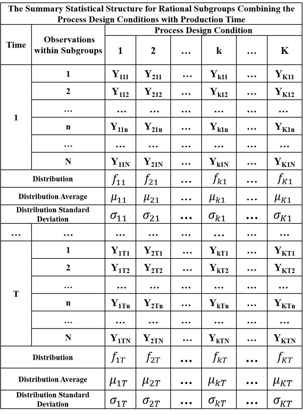
Figure 10-5. The Statistical Structure for SDS = 1
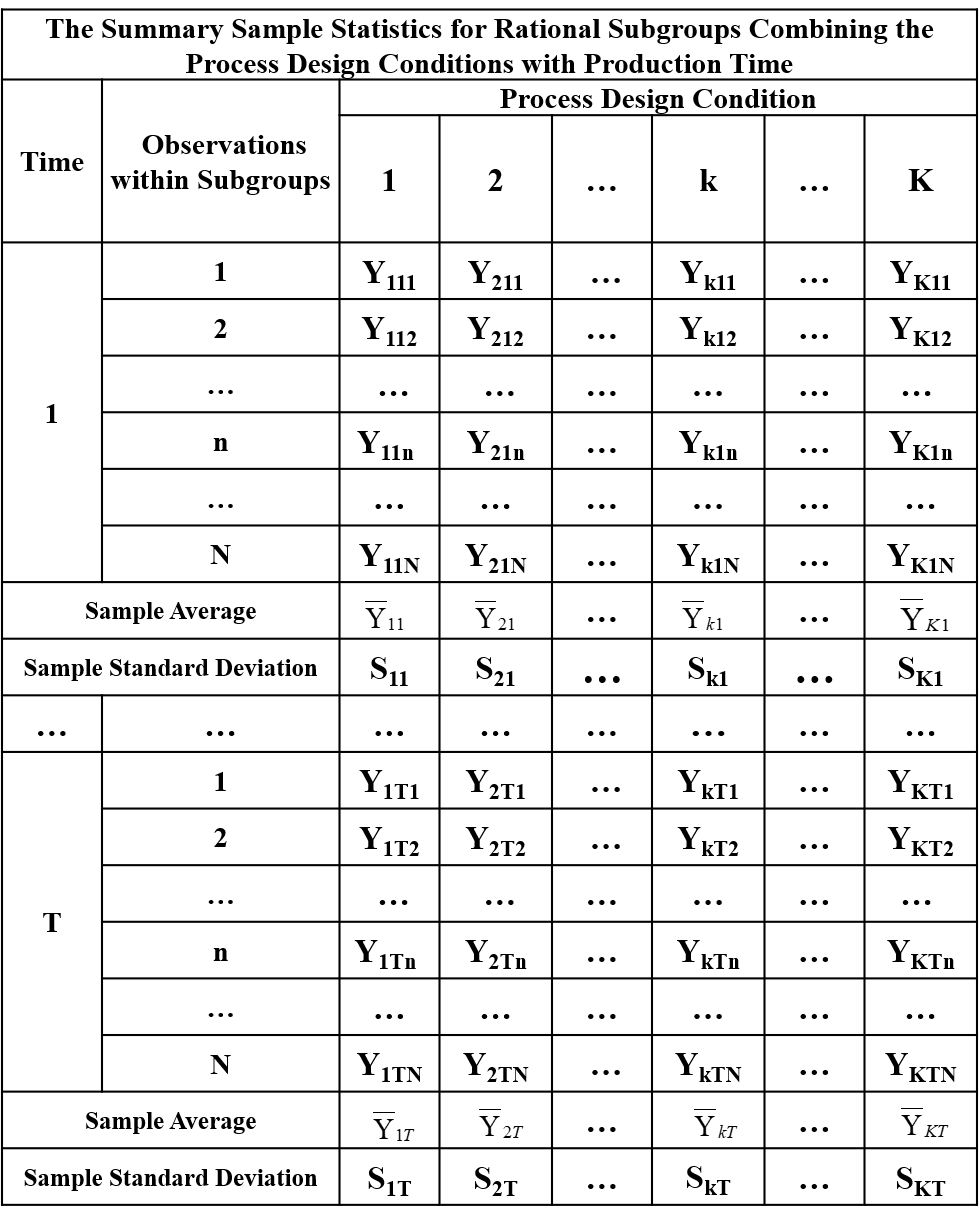
Figure 10-6. The RSG Sample Statistics for SDS = 1
The rational subgroup means are estimated by the rational subgroup sample means as in Equation 10-7.
(equation picture — LaTeX to be added)
Equation 10-7. Estimate for µkt
For SDS = 1 all the rational subgroups , and the rational subgroup standard deviations are estimated by the sample standard deviations given in Equation 10-8.
(equation picture — LaTeX to be added)
Equation 10-8. Estimate for σkt
The re-parameterized statistical model parameters are parametric functions of the fundamental rational subgroup means . Therefore the estimates of these model parameters are direct functions of the rational subgroup sample means as shown in Equation 10-9.
(equation picture — LaTeX to be added)
Equation 10-9. Estimates for the Re-Parameterized VAS Model Parameters
10.6.1 Estimation of the Model Error Terms
The method of estimating the model error terms depends upon the sampling design state, and is very important component of the VAS methodology that is discussed in more detail in later chapters. But, for any rational subgrouping structure where for all of the rational subgroups, the error terms are estimated as in Equation 10-10.
Equation 10-10. The Error Term for SDS = 1
10.7 The Distribution of the Sample Average
The following well-known deductively valid theorems regarding the distribution of the sample average come from probability theory.[33]
Theorem 1: If {, , … , }is a random sample of size N from a constant cause system that is that is described by a normal distribution with mean µ and standard deviation σ, then the sample average will be normally distributed with mean and standard deviation .
Theorem 2: If {, , … , }is a random sample of size N from a constant cause system described by any distribution that admits a mean µ and standard deviation σ, then the mean for the distribution of sample averages is and the standard deviation for the distribution of sample averages is .
Theorem 3 (The Central Limit Theorem): If {, , … , }is a random sample of size N from a constant cause system described by any distribution with mean µ and standard deviation σ, then as the distribution for sample average converges to the normal distribution with mean and standard deviation .
10.8 The Distribution of the Sample Standard Deviation
The distribution for the sample standard deviation S is only known for the case where a random sample {, , … ,} is drawn from a distribution.[34] In this case the mean for the distribution of the sample standard deviation S is given in Equation 10-11.
Equation 10-11. The Mean for the Distribution of S
where
and the Gamma function is
The value of the constant is less than 1 which means the sample standard deviation S underestimates . The constant is often referred to as the “bias correction factor” because an unbiased estimate for is given by Equation 10-12.
Equation 10-12. The Unbiased Estimate for σ
The standard deviation for the distribution of the sample standard deviation S is given by Equation 10-13.
Equation 10-13. The Standard Deviation for the Distribution of S
An unbiased estimate for is given by Equation 10-14.
Equation 10-14. The Unbiased Estimate for σS
10.9 Chebyshev’s Theorem
Dr. Shewhart’s claim regarding the efficiency of the sample average and standard deviation as the basis for our analysis is reinforced by the application of Chebyshev’s theorem. This theorem is a very famous and important deductively valid theorem in statistics that is often misunderstood by practitioners.[35] The formal statement of Chebyshev’s theorem is the following.
If the performance measurement Y is produced by a constant cause system described by a density function f with mean µ and finite standard deviation σ, then for every value of k > 1
or
Chebyshev’s theorem tells us that for any constant cause system of variation that has a finite standard deviation σ, the individual values for the performance measurement Y generated by the cause system cannot fall arbitrarily far away from the distribution mean µ. This statement is true, and this is very important, no matter what the form of the underlying density function f as long as f admits the existence of a standard deviation which is almost always the case in practice. The use of this theorem often allows us to dispense with the traditional assumption that the underlying statistical distribution is a “normal distribution”.
Applying Chebyshev’s theorem, we can make the following claims which are graphically illustrated in Figure 10-7.
At least 75% of the observations generated from a constant cause system of variation will fall within 2 standard deviation units of the mean.
At least 89% of the observations generated from a constant cause system of variation will fall within 3 standard deviation units of the mean.
At least 94% of the observations generated from a constant cause system of variation will fall within 4 standard deviation units of the mean.
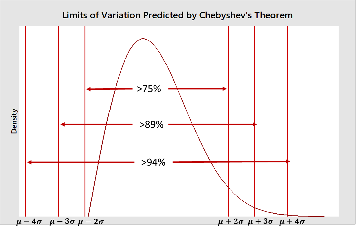
Figure 10-7. The Range of Variation for Constant Cause Systems of Variation
Many theoretical and simulation studies have demonstrated that the bounds obtained from the Chebyshev theorem are actually very conservative. In most applications the percentages associated the 2, 3 and 4 sigma limits are much higher.
Now in any actual application the statistical distribution function f, and the values for , are unknown to the analyst. These values must be estimated using a sample selected from the cause system under study. The limits in Chebyshev’s theorem are then estimated by replacing with the sample average and the standard deviation σ with the sample standard deviation S. So, for example, the 3-sigma limits are those in Equation 10-15.
Equation 10-15. The Estimated 3-Sigma Limits
The empirical intervals based on the sample data can be used to predict the range of variation expected in the future data produced by the constant cause system from which the sample was drawn based on the assumption “the future behaves like the past”. Because these intervals are not based on theory, but on sample data, we refer to these intervals as “empirical intervals”, and the probability statements associated with these intervals are collectively referred to as the “empirical rule”.
Such pitfalls exist for any method of analysis used in practice.
The “Dot Notation” refers to the summation over the indices where the dot occurs. This notation is taken directly from page 56 of the book The Analysis of Variance by Henry Scheffe and is used to simplify and clarify the summation processes required to calculate the parameter estimates.
See the note on page 646 of Applied Linear Statistical Models by Neter and Wasserman where they address this issue.
For an in-depth discussion of the distributions for the sample mean and sample standard deviation refer to the book The Scientific Basis for Modern Analytic Practice by Dr. Thomas Bishop.
The detailed derivation of the theory for the distribution of S for the normal distribution can be found in Chapter 11 of the book Statistical Theory with Engineering Applications by A. Hald.
For a detailed discussion on this point the reader is referred to Section 15.8 in the book The Scientific Basis for Modern Analytic Practice by Dr. Thomas Bishop.