9.0 The Sampling Plan and Sampling Design States
The problem formulation leads to the set of R = KxT rational subgroups defined by the combinations of the process design conditions and production times. The conceptual structure of the data based on the problem formulation is presented in Figure 9-1.
The complete analysis of the causes creating the variation in the performance measurement across the rational subgroups depends on our ability to estimate all of the rational subgroup means and standard deviations . The desired estimates of these parameters are described in Equation 9-1 and Equation 9-2. But at least one observation is required to calculate the sample mean , and at least two observations are required to calculate the sample standard deviation .
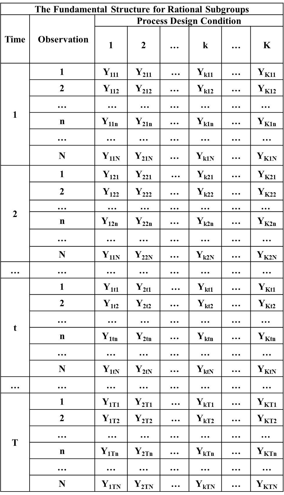
Figure 9-1. The Data Structure Based on the Problem Formulation
Equation 9-1. Rational Subgroup Sample Average
and
Equation 9-2. Rational Subgroup Sample Standard Deviation
9.1 The Sampling Plan
Once the problem formulation is completed, a sampling plan is executed to produce the data within the rational subgroups. The sampling plan involves the collection of these data using either statistical samples, a designed experiment, a transactional or observational study, or a judgment or convenience sample.
9.2 The Sampling Design States
While the data structure in Figure 9-1 is desired, in practice once the sampling plan is executed there may be rational subgroups containing only a single observation (i.e. ) or subgroups with no observations (i.e. ). In these cases some of the rational subgroup means and/or the standard deviations cannot be estimated.
The actual data structure within and across the rational subgroups resulting from the execution of the sampling plan is associated with a “sampling design state (SDS)” which is defined by the values of the rational subgroup sample sizes . Knowledge of the sampling design state is very important because it alerts the analyst to cases where some of the rational subgroup means and/or the standard deviations cannot be estimated. In these cases the effects of some of the process design conditions and/or production times will be missed in the analysis.
9.2.1 Complete, Semi-Complete and Incomplete Sampling Design States
A sampling design state is said to be “complete” if for each of the rational subgroups. For this sampling design state all of the rational subgroup means , and all of the rational subgroup standard deviations , can be estimated using the rational subgroup sample means and sample standard deviations.
A sampling design state is said to be “semi-complete” if the samples size for all of the rational subgroups, or the samples size for some of the rational subgroups and for the remaining rational subgroups. In these cases all of the rational subgroup means can be estimated, but not all of the rational subgroup standard deviations can be estimated. So in this case we are lacking information on the range of variation within those rational subgroups where .
A sampling design state is said to be “incomplete” if the sample size for one or more of the rational subgroups. When there is no information available about the statistical properties of the data produced within the rational subgroup. In this case our information on the statistical properties with respect to all of the R=KxT rational subgroups is incomplete.
9.2.2 The Six Sampling Design States
There are six possible sampling design states which are described in Table 9-1.
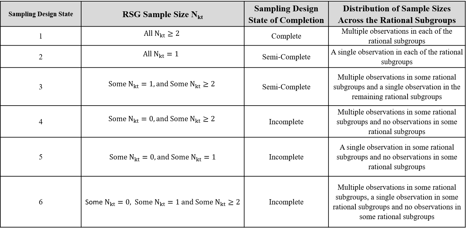
Table 9-1. The Six Sampling Design States
Sampling design state 1 is the complete and preferred state, and the data structure for this state is presented in Figure 9-2.
Sampling design state 2 is an important “semi-complete” design state which occurs often in practice. In this state there is a single observation within each rational subgroup (i.e. for each rational subgroup). The data structure for this important sampling design state is presented in Figure 9-3. In this state none of the rational subgroup standard deviations can be directly estimated, and an alternative, approximate method must be employed to analyze the unexplained causes of variation.
In sampling design state 3 the sample size for some of the rational subgroups, and the remaining sample sizes are . This sampling design state is illustrated in Figure 9-4.
In sampling design state 4 the sample size for some of the rational subgroups, and for the remaining rational subgroups. This sampling design state is illustrated in Figure 9-5. While this is an “incomplete” sampling design state it is often purposely used by analysts in experimental settings to reduce the amount of sampling required to study the effects of the process design conditions and production time on the performance measurement of interest. One example where this is achieved is by rotating the sampling across the process design conditions over time using sample sizes .
Sampling design states 5 and 6 can be very incomplete sampling design states. These design states are illustrated in Figure 9-6 and Figure 9-7.
9.3 Sparse Datasets - A Caution
It is extremely important to understand that the VAS methodology is primarily designed to handle studies involving sampling design states 1 and 2, and sampling design state 4 when 4 is chosen by the analyst as part of a designed experiment. The sampling design states 4, 5 and 6 are incomplete, and associated with “sparse” data associated with rational subgroups where and .
In some applications these sampling design states may still provide valuable insights on the effects of the process design conditions and/or production time on the variation in the performance measurement. But when these sampling design states result outside the control of the analyst, the data may be so sparse that significant biases and misleading information can be produced by the analysis. It is also possible that the data are so sparse as to make the analysis impossible. So in almost all cases the use of these incomplete sampling design states is risky and should be viewed with caution if they form the basis for the analysis.
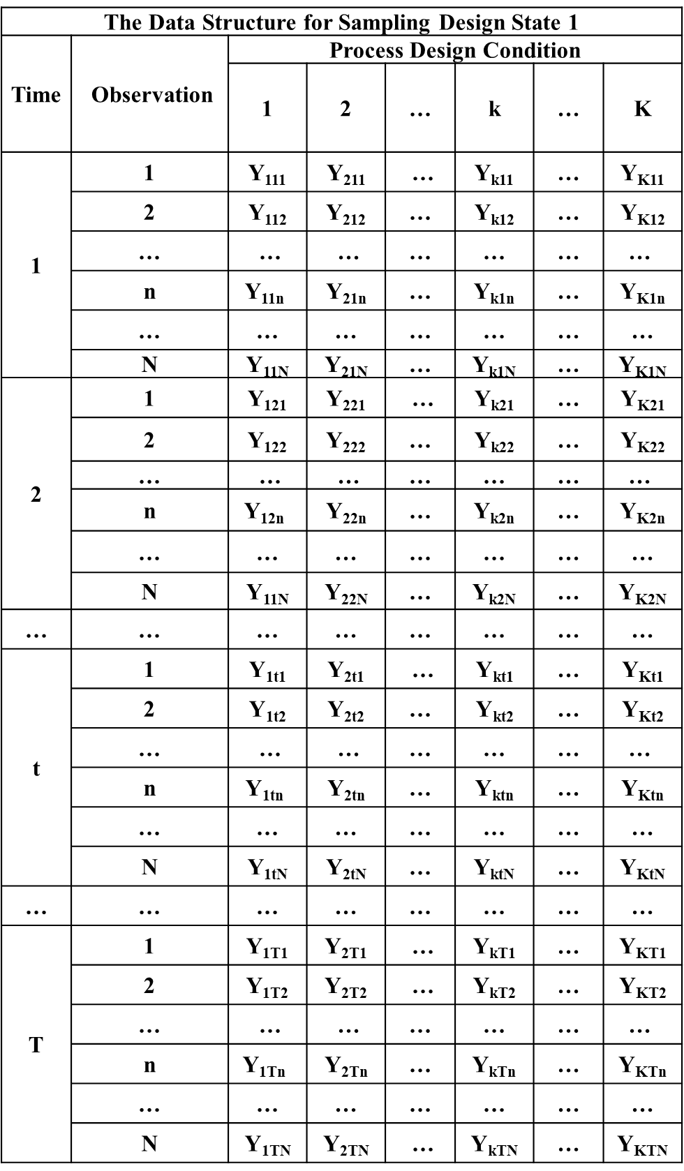
Figure 9-2. Data Structure for Sampling Design State 1
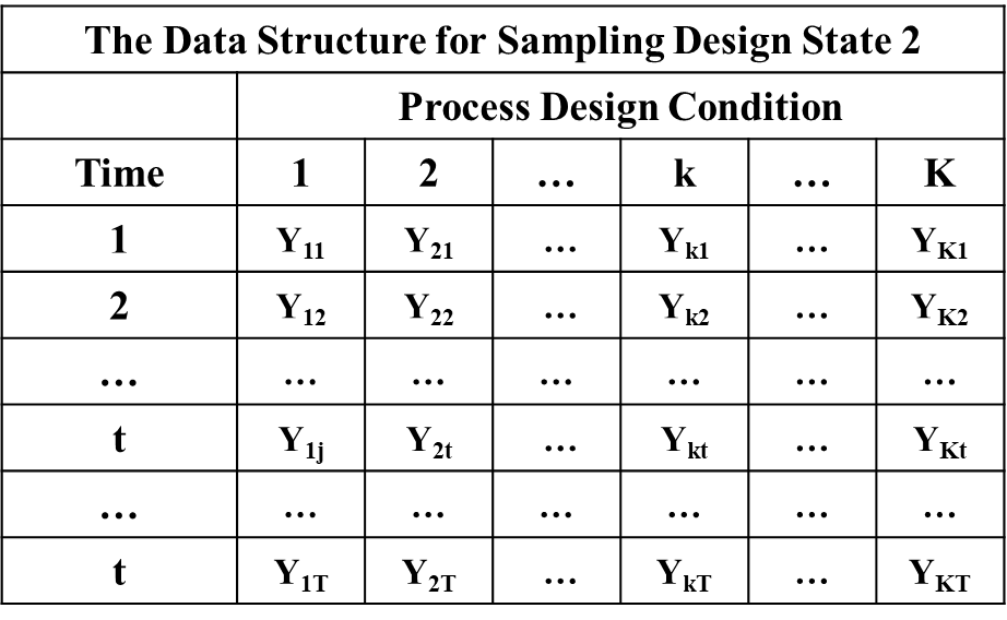
Figure 9-3. Data Structure for Sampling Design State 2
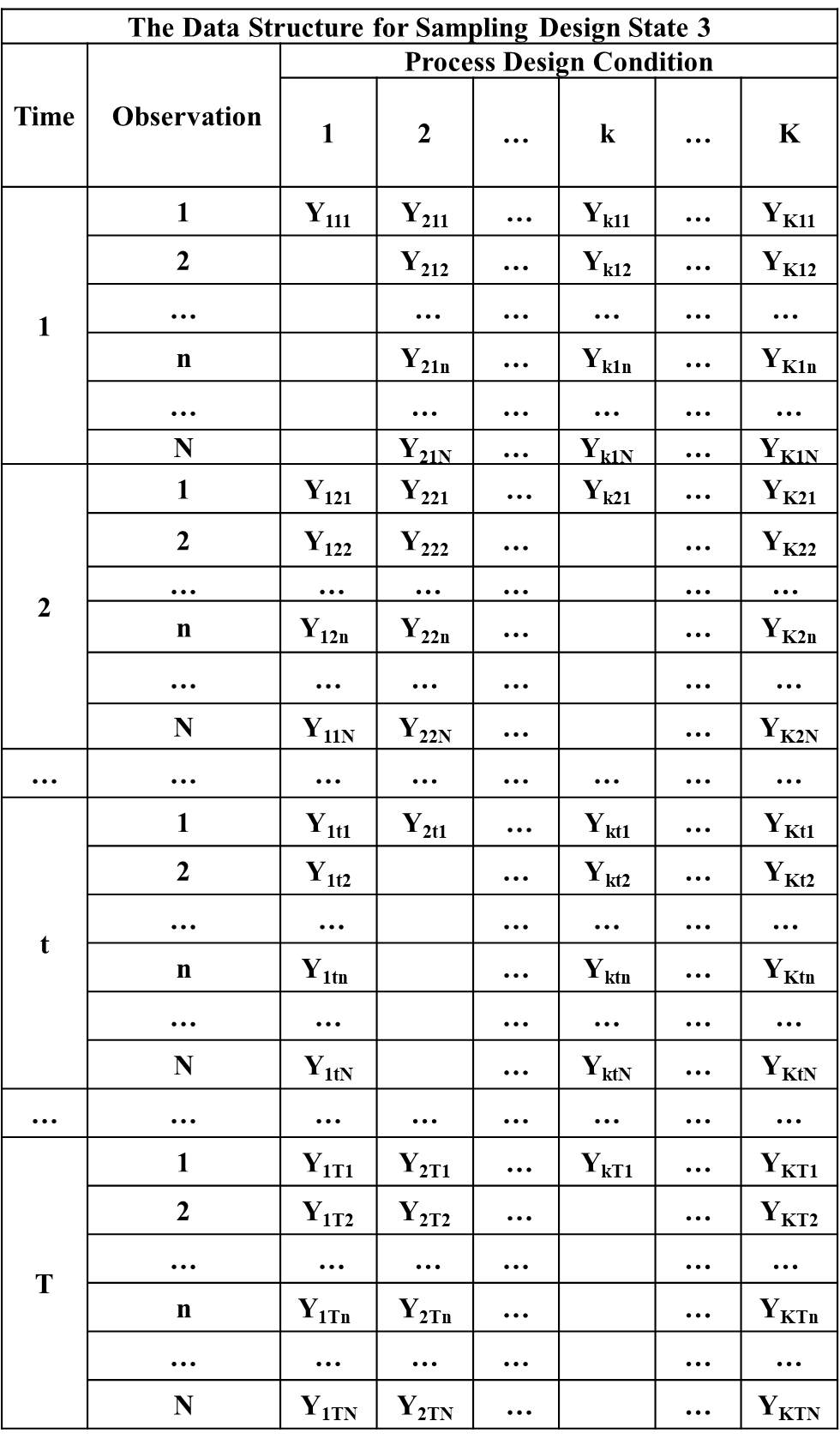
Figure 9-4. Data Structure for Sampling Design State 3
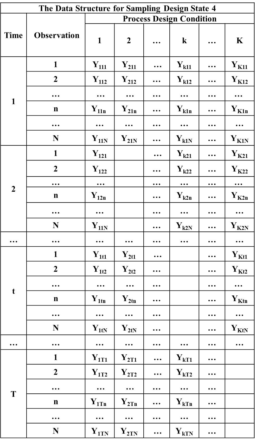
Figure 9-5. Data Structure for Sampling Design State 4
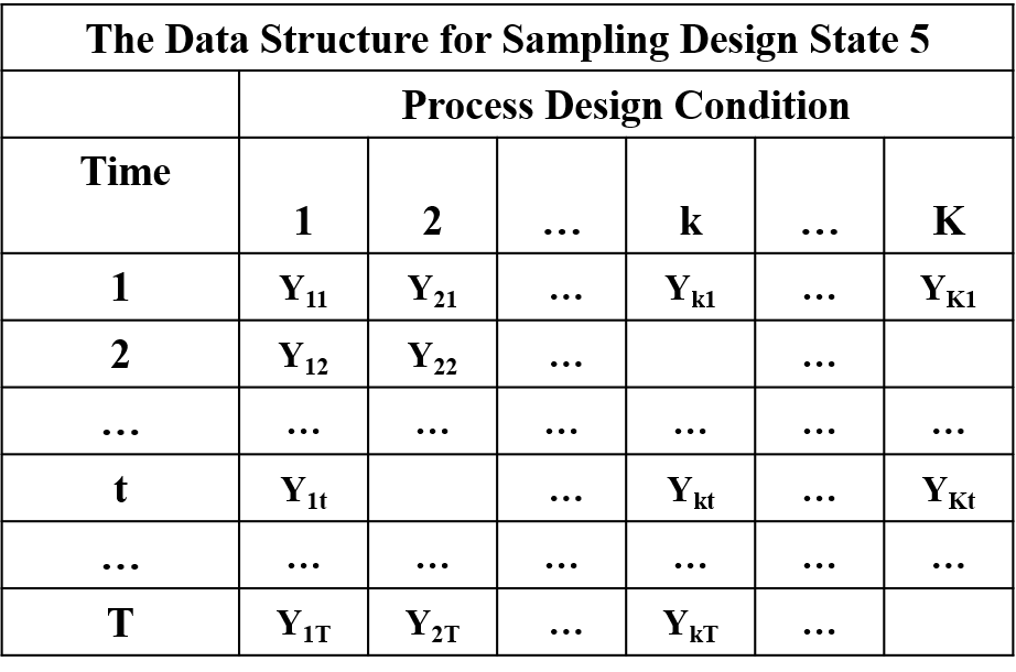
Figure 9-6. Data Structure for Sampling Design State 5
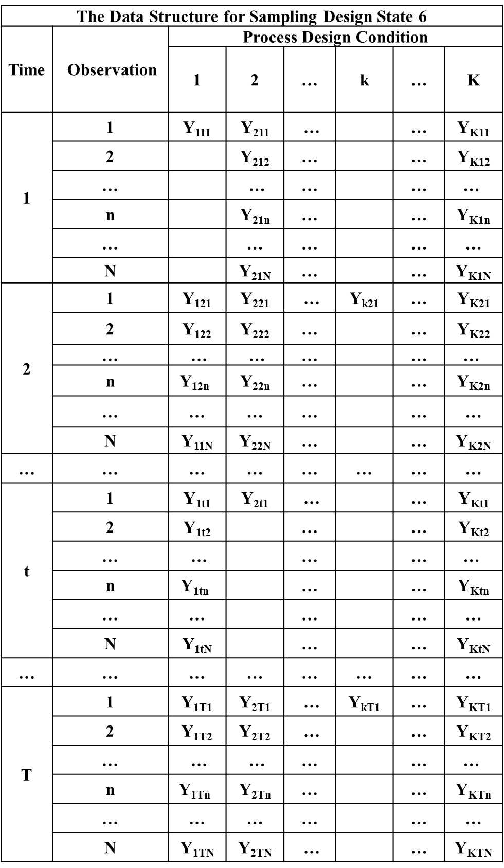
Figure 9-7. Data Structure for Sampling Design State 6